14.451 Lecture Notes Economic Growth

More documents

Recommendations

Info

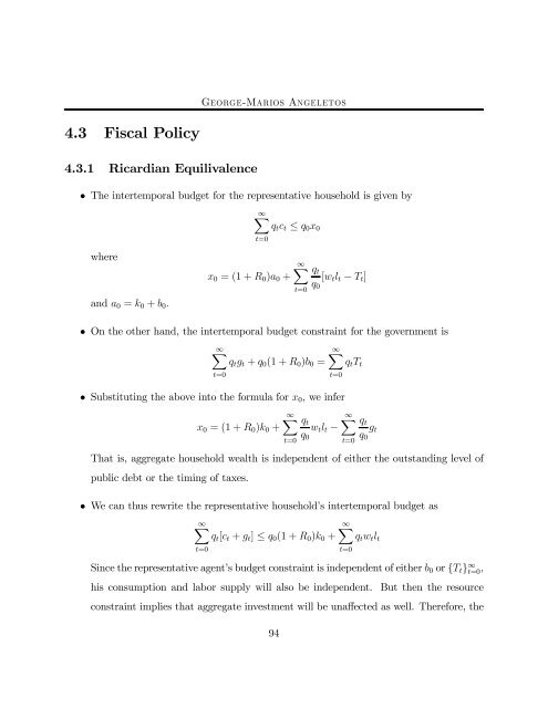
4.3 Fiscal Policy 4.3.1 Ricardian Equilivalence George-Marios Angeletos • The intertemporal budget for the representative household is given by where and a0 = k0 + b0. ∞X t=0 x0 =(1+R0)a0 + qtct ≤ q0x0 ∞X t=0 qt q0 [wtlt − Tt] • On the other hand, the intertemporal budget constraint for the government is ∞X qtgt + q0(1 + R0)b0 = • Substituting the above into the formula for x0, we infer t=0 x0 =(1+R0)k0 + ∞X ∞X t=0 qtTt ∞X qt qt wtlt − gt q0 q0 t=0 t=0 That is, aggregate household wealth is independent of either the outstanding level of public debt or the timing of taxes. • We can thus rewrite the representative household’s intertemporal budget as ∞X qt[ct + gt] ≤ q0(1 + R0)k0 + t=0 ∞X t=0 qtwtlt Since the representative agent’s budget constraint is independent of either b0 or {Tt} ∞ t=0, his consumption and labor supply will also be independent. But then the resource constraint implies that aggregate investment will be unaffected as well. Therefore, the 94
14.451 Lecture Notes aggregate path {ct,kt} ∞ t=0 is independent of either b0 or {Tt} ∞ t=0. All that matter is the stream of government spending, not the way this is financed. • More generally, consider now arbitrary preferences and endogenous labor supply, but suppose that the tax burden and public debt is uniformly distributed across households. Then, for every individual j, effective wealth is independent of either the level of public debt or the timing of taxes: ∞X x j 0 =(1+R0)k j 0 + t=0 qt q0 ∞X wtl j t − t=0 Since the individual’s intertemporal budget is independent of either b0 or {Tt} ∞ t=0, her optimal plan {c j t,l j t,a j t} ∞ t=0 will also be independent of either b0 or {Tt} ∞ t=0 for any given price path. But if individual behavior does not change for given prices, markets will continue to clear for the same prices. That is, equilibrium prices are indeed also independent of either b0 or {Tt} ∞ t=0. We conclude Proposition 21 Equilibrium prices and allocations are independent of either the intial level of public debt, or the mixture of deficits and (lump-sum) taxes that the government uses to finance governement spending. • Remark: For Ricardian equivalence to hold, it is critical both that markets are complete (so that agents can freely trade the riskless bond) and that horizons are infinite (so that the present value of taxes the household expects to pay just equals the amount of public debt it holds). If either condition fails, such as in OLG economies or economies with borrowing constraints, Ricardian equivalence will also fail. Ricardian equivalence may also fail if there are 95 qt q0 gt,
Page 1 and 2:
14.451 Lecture Notes Economic Growt
Page 3 and 4:
Contents Preface ix 1 Introduction
Page 5 and 6:
14.451 Lecture Notes 3.1.4 OptimalC
Page 7 and 8:
14.451 Lecture Notes 5.2 SomeExampl
Page 9 and 10:
Preface This is the set of lecture
Page 11 and 12:
Chapter 1 IntroductionandGrowthFact
Page 13 and 14:
14.451 Lecture Notes 1.2 The World
Page 15 and 16:
14.451 Lecture Notes • Figure 4 3
Page 17 and 18:
14.451 Lecture Notes 9. Openness: I
Page 19 and 20:
Chapter 2 The Solow Growth Model (a
Page 21 and 22:
14.451 Lecture Notes • We say tha
Page 23 and 24:
14.451 Lecture Notes 2.1.3 The Reso
Page 25 and 26:
whereas consumption is given by 14.
Page 27 and 28:
14.451 Lecture Notes where the latt
Page 29 and 30:
14.451 Lecture Notes 2.2 Decentrali
Page 31 and 32:
14.451 Lecture Notes • Let K m t
Page 33 and 34:
Equivalently, 14.451 Lecture Notes
Page 35 and 36:
14.451 Lecture Notes where Kt ≡ R
Page 37 and 38:
14.451 Lecture Notes Proof. Follows
Page 39 and 40:
14.451 Lecture Notes • Combining
Page 41 and 42:
14.451 Lecture Notes We would expec
Page 43 and 44:
• Straightforward algebra gives W
Page 45 and 46:
14.451 Lecture Notes • Suppose th
Page 47 and 48:
2.6 Miscellaneous 14.451 Lecture No
Page 49 and 50:
14.451 Lecture Notes 2.6.3 Introduc
Page 51 and 52:
Chapter 3 The Neoclassical Growth M
Page 53 and 54: 14.451 Lecture Notes ut+1 : There i
Page 55 and 56: 14.451 Lecture Notes • Combining
Page 57 and 58: Equivalently, taking (kt,kt+2) as g
Page 59 and 60: equivalently 14.451 Lecture Notes
Page 61 and 62: 14.451 Lecture Notes • Let B be t
Page 63 and 64: 14.451 Lecture Notes 3.2 Decentrali
Page 65 and 66: 14.451 Lecture Notes only the total
Page 67 and 68: 14.451 Lecture Notes • Finally, i
Page 69 and 70: 14.451 Lecture Notes The constraint
Page 71 and 72: 14.451 Lecture Notes where f(k) ≡
Page 73 and 74: 14.451 Lecture Notes Proposition 15
Page 75 and 76: 14.451 Lecture Notes individual’s
Page 77 and 78: 14.451 Lecture Notes 3.3 Steady Sta
Page 79 and 80: 3.3.2 Transitional Dynamics 14.451
Page 81 and 82: 14.451 Lecture Notes Proof. The pol
Page 83 and 84: 14.451 Lecture Notes • The ˙c =0
Page 85 and 86: 14.451 Lecture Notes 3.5 Comparativ
Page 87 and 88: 14.451 Lecture Notes • We conclud
Page 89 and 90: where At denotes TFP. Note that 14.
Page 91 and 92: 14.451 Lecture Notes • Note that
Page 93 and 94: 14.451 Lecture Notes 3.6.2 Impulse
Page 95 and 96: Chapter 4 Applications 4.1 Arrow-De
Page 97 and 98: 14.451 Lecture Notes bles. We can t
Page 99 and 100: 14.451 Lecture Notes • Then, the
Page 101 and 102: 14.451 Lecture Notes • More gener
Page 103: 14.451 Lecture Notes • Consider n
Page 107 and 108: 14.451 Lecture Notes notes to be co
Page 109 and 110: Chapter 5 Overlapping Generations M
Page 111 and 112: 14.451 Lecture Notes Life-cycle con
Page 113 and 114: Note that Recall that ∂m ∂R 14.
Page 115 and 116: where the scalar ζ>0 is given by 1
Page 117 and 118: 14.451 Lecture Notes • Finally, n
Page 119 and 120: Chapter 6 Endogenous Growth I: AK,
Page 121 and 122: 14.451 Lecture Notes so that consum
Page 123 and 124: 14.451 Lecture Notes • Finally, t
Page 125 and 126: 14.451 Lecture Notes • Combining
Page 127 and 128: 14.451 Lecture Notes Like in the si
Page 129 and 130: 14.451 Lecture Notes Combining the
Page 131 and 132: 14.451 Lecture Notes • Households
Page 133 and 134: 14.451 Lecture Notes Proposition 25
Page 135 and 136: Chapter 7 Endogenous Growth II: R&D
Page 137 and 138: 14.451 Lecture Notes More generally
Page 139 and 140: 14.451 Lecture Notes you can think
Page 141 and 142: 14.451 Lecture Notes Free entry in
Page 143 and 144: 14.451 Lecture Notes 7.1.8 Pareto A
Page 145 and 146: 14.451 Lecture Notes 7.1.9 Introduc
Page 147 and 148: 7.2.2 The Value of Innovation 14.45
Page 149 and 150: 14.451 Lecture Notes It follows tha
Page 151 and 152: 14.451 Lecture Notes • Compare no
show all

14.451 Lecture Notes Economic Growth

Create successful ePaper yourself

Delete template?

Save as template?