14.451 Lecture Notes Economic Growth
14.451 Lecture Notes Economic Growth
14.451 Lecture Notes Economic Growth
You also want an ePaper? Increase the reach of your titles
YUMPU automatically turns print PDFs into web optimized ePapers that Google loves.
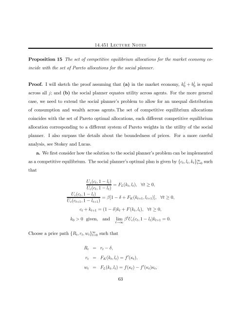
<strong>14.451</strong> <strong>Lecture</strong> <strong>Notes</strong><br />
Proposition 15 The set of competitive equilibrium allocations for the market economy co-<br />
incide with the set of Pareto allocations for the social planner.<br />
Proof. I will sketch the proof assuming that (a) in the market economy, k j<br />
0 + b j<br />
0 is equal<br />
across all j; and (b) the social planner equates utility across agents. For the more general<br />
case, we need to extend the social planner’s problem to allow for an unequal distribution<br />
of consumption and wealth across agents. The set of competitive equilibrium allocations<br />
coincides with the set of Pareto optimal allocations, each different competitive equilibrium<br />
allocation corresponding to a different system of Pareto weights in the utility of the social<br />
planner. I also surpass the details about the boundedness of prices. For a more careful<br />
analysis, see Stokey and Lucas.<br />
a. We first consider how the solution to the social planner’s problem can be implemented<br />
as a competitive equilibrium. The social planner’s optimal plan is given by {ct,lt,kt} ∞ t=0 such<br />
that<br />
Uz(ct, 1 − lt)<br />
Uc(ct, 1 − lt) = FL(kt,lt), ∀t ≥ 0,<br />
Uc(ct, 1 − lt)<br />
Uc(ct+1, 1 − lt+1) = β[1 − δ + FK(kt+1,lt+1)], ∀t ≥ 0,<br />
ct + kt+1 =(1− δ)kt + F (kt,lt), ∀t ≥ 0,<br />
k0 > 0 given, and lim<br />
t→∞ β t Uc(ct, 1 − lt)kt+1 =0.<br />
Choose a price path {Rt,rt,wt} ∞ t=0 such that<br />
Rt = rt − δ,<br />
rt = FK(kt,lt) =f 0 (κt),<br />
wt = FL(kt,lt) =f(κt) − f 0 (κt)κt,<br />
63


