14.451 Lecture Notes Economic Growth

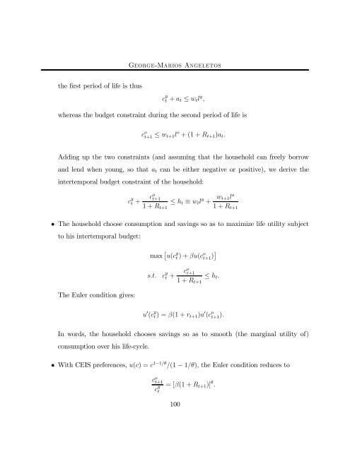
the first period of life is thus
George-Marios Angeletos
c y
t + at ≤ wtl y ,
whereas the budget constraint during the second period of life is
c o t+1 ≤ wt+1l o +(1+Rt+1)at.
Adding up the two constraints (and assuming that the household can freely borrow
and lend when young, so that at can be either negative or positive), we derive the
intertemporal budget constraint of the household:
c y
t + co t+1
1+Rt+1
≤ ht ≡ wtl y o
wt+1l
+
1+Rt+1
• The household choose consumption and savings so as to maximize life utility subject
to his intertemporal budget:
The Euler condition gives:
max £ u(c y
t )+βu(c o t+1 )¤
s.t. c y
t + co t+1
1+Rt+1
≤ ht.
u 0 (c y
t )=β(1 + rt+1)u 0 (c o t+1).
In words, the household chooses savings so as to smooth (the marginal utility of)
consumption over his life-cycle.
• With CEIS preferences, u(c) =c 1−1/θ /(1 − 1/θ), the Euler condition reduces to
c o t+1
c y
t
=[β(1 + Rt+1)] θ .
100