14.451 Lecture Notes Economic Growth

14.451 Lecture Notes
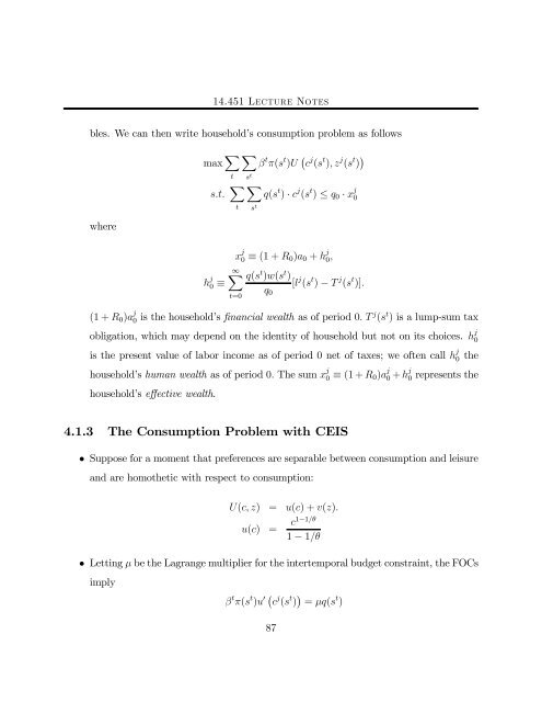
bles. We can then write household’s consumption problem as follows
max X X
β t π(s t )U ¡ c j (s t ),z j (s t ) ¢
where
t
s t
s.t. X X
t
h j
0 ≡
t=0
s t
q(s t ) · c j (s t ) ≤ q0 · x j
0
x j
0 ≡ (1 + R0)a0 + h j
∞X
0,
q(st )w(st )
[l
q0
j (s t ) − T j (s t )].
(1 + R0)a j
0 is the household’s financial wealth as of period 0. Tj (st ) is a lump-sum tax
obligation, which may depend on the identity of household but not on its choices. h j
0
is the present value of labor income as of period 0 net of taxes; we often call h j
0 the
household’s human wealth as of period 0. The sum x j
0 ≡ (1 + R0)a j
0 + h j
0 represents the
household’s effective wealth.
4.1.3 The Consumption Problem with CEIS
• Suppose for a moment that preferences are separable between consumption and leisure
and are homothetic with respect to consumption:
U(c, z) = u(c)+v(z).
u(c) = c1−1/θ
1 − 1/θ
• Letting µ be the Lagrange multiplier for the intertemporal budget constraint, the FOCs
imply
β t π(s t )u 0 ¡ c j (s t ) ¢ = µq(s t )
87