14.451 Lecture Notes Economic Growth

14.451 Lecture Notes
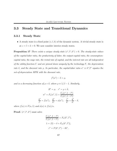
3.3 Steady State and Transitional Dynamics
3.3.1 Steady State
• A steady state is a fixed point (c, l, k) of the dynamic system. A trivial steady state is
at c = l = k =0. We now consider interior steady states.
Proposition 17 There exists a unique steady state (c ∗ ,l ∗ ,k ∗ ) > 0. The steady-state values
of the capital-labor ratio, the productivity of labor, the output-capital ratio, the consumption-
capital ratio, the wage rate, the rental rate of capital, and the interest rate are all independent
of the utility function U and are pinned down uniquely by the technology F , the depreciation
rate δ, andthediscountrateρ. In particular, the capital-labor ratio κ ∗ ≡ k ∗ /l ∗ equates the
net-of-depreciation MPK with the discount rate,
f 0 (κ ∗ ) − δ = ρ,
and is a decreasing function of ρ + δ, where ρ ≡ 1/β − 1. Similarly,
R ∗ = ρ, r ∗ = ρ + δ,
w ∗ = FL(κ ∗ , 1) = Uz(c ∗ , 1 − l ∗ )
Uc(c ∗ , 1 − l ∗ ) ,
y ∗
l ∗ = f(κ∗ ),
where f(κ) ≡ F (κ, 1) and φ(κ) ≡ f(κ)/κ.
Proof. (c ∗ ,l ∗ ,k ∗ ) must solve
y ∗
k ∗ = φ(κ∗ ),
c ∗
k
∗ = y∗
Uz(c ∗ , 1 − l ∗ )
Uc(c ∗ , 1 − l ∗ ) = FL(k ∗ ,l ∗ ),
1=β[1 − δ + FK(k ∗ ,l ∗ )],
c ∗ = F (k ∗ ,l ∗ ) − δk ∗ ,
67
− δ,
k∗