Basic Tools for Process Improvement
Basic Tools for Process Improvement
Basic Tools for Process Improvement

Create successful ePaper yourself
Turn your PDF publications into a flip-book with our unique Google optimized e-Paper software.
<strong>Basic</strong> <strong>Tools</strong> <strong>for</strong> <strong>Process</strong> <strong>Improvement</strong><br />
Module 11<br />
HISTOGRAM<br />
HISTOGRAM 1
What is a Histogram?<br />
<strong>Basic</strong> <strong>Tools</strong> <strong>for</strong> <strong>Process</strong> <strong>Improvement</strong><br />
A Histogram is a vertical bar chart that depicts the distribution of a set of data. Unlike<br />
Run Charts or Control Charts, which are discussed in other modules, a Histogram<br />
does not reflect process per<strong>for</strong>mance over time. It's helpful to think of a Histogram<br />
as being like a snapshot, while a Run Chart or Control Chart is more like a movie<br />
(Viewgraph 1).<br />
When should we use a Histogram?<br />
When you are unsure what to do with a large set of measurements presented in a<br />
table, you can use a Histogram to organize and display the data in a more userfriendly<br />
<strong>for</strong>mat. A Histogram will make it easy to see where the majority of values<br />
falls in a measurement scale, and how much variation there is. It is helpful to<br />
construct a Histogram when you want to do the following (Viewgraph 2):<br />
! Summarize large data sets graphically. When you look at Viewgraph 6,<br />
you can see that a set of data presented in a table isn’t easy to use. You can<br />
make it much easier to understand by summarizing it on a tally sheet<br />
(Viewgraph 7) and organizing it into a Histogram (Viewgraph 12).<br />
! Compare process results with specification limits. If you add the<br />
process specification limits to your Histogram, you can determine quickly<br />
whether the current process was able to produce "good" products.<br />
Specification limits may take the <strong>for</strong>m of length, weight, density, quantity of<br />
materials to be delivered, or whatever is important <strong>for</strong> the product of a given<br />
process. Viewgraph 14 shows a Histogram on which the specification limits,<br />
or "goalposts," have been superimposed. We’ll look more closely at the<br />
implications of specification limits when we discuss Histogram interpretation<br />
later in this module.<br />
! Communicate in<strong>for</strong>mation graphically. The team members can easily<br />
see the values which occur most frequently. When you use a Histogram to<br />
summarize large data sets, or to compare measurements to specification<br />
limits, you are employing a powerful tool <strong>for</strong> communicating in<strong>for</strong>mation.<br />
! Use a tool to assist in decision making. As you will see as we move<br />
along through this module, certain shapes, sizes, and the spread of data have<br />
meanings that can help you in investigating problems and making decisions.<br />
But always bear in mind that if the data you have in hand aren’t recent, or you<br />
don’t know how the data were collected, it’s a waste of time trying to chart<br />
them. Measurements cannot be used <strong>for</strong> making decisions or predictions<br />
when they were produced by a process that is different from the current one,<br />
or were collected under unknown conditions.<br />
2 HISTOGRAM
100<br />
80<br />
60<br />
40<br />
20<br />
0<br />
<strong>Basic</strong> <strong>Tools</strong> <strong>for</strong> <strong>Process</strong> <strong>Improvement</strong><br />
What Is a Histogram?<br />
0 5 10 15 20 25 30 35 40 45 50 55 60<br />
• A bar graph that shows the distribution of data<br />
• A snapshot of data taken from a process<br />
HISTOGRAM VIEWGRAPH 1<br />
When Are Histograms Used?<br />
• Summarize large data sets graphically<br />
• Compare measurements to specifications<br />
• Communicate in<strong>for</strong>mation to the team<br />
• Assist in decision making<br />
HISTOGRAM VIEWGRAPH 2<br />
HISTOGRAM 3
<strong>Basic</strong> <strong>Tools</strong> <strong>for</strong> <strong>Process</strong> <strong>Improvement</strong><br />
What are the parts of a Histogram?<br />
As you can see in Viewgraph 3, a Histogram is made up of five parts:<br />
1. Title: The title briefly describes the in<strong>for</strong>mation that is contained in the<br />
Histogram.<br />
2. Horizontal or X-Axis: The horizontal or X-axis shows you the scale of<br />
values into which the measurements fit. These measurements are generally<br />
grouped into intervals to help you summarize large data sets. Individual data<br />
points are not displayed.<br />
3. Bars: The bars have two important characteristics—height and width. The<br />
height represents the number of times the values within an interval occurred.<br />
The width represents the length of the interval covered by the bar. It is the<br />
same <strong>for</strong> all bars.<br />
4. Vertical or Y-Axis: The vertical or Y-axis is the scale that shows you the<br />
number of times the values within an interval occurred. The number of times<br />
is also referred to as "frequency."<br />
5. Legend: The legend provides additional in<strong>for</strong>mation that documents where<br />
the data came from and how the measurements were gathered.<br />
4 HISTOGRAM
4<br />
5<br />
F<br />
R<br />
E<br />
Q<br />
U<br />
E<br />
N<br />
C<br />
Y<br />
100<br />
80<br />
60<br />
40<br />
20<br />
<strong>Basic</strong> <strong>Tools</strong> <strong>for</strong> <strong>Process</strong> <strong>Improvement</strong><br />
Parts of a Histogram<br />
DAYS OF OPERATION PRIOR TO<br />
FAILURE FOR AN HF RECEIVER<br />
0<br />
0 5 10 15 20 25 30 35 40 45 50 55 60<br />
DAYS OF OPERATION<br />
MEAN TIME BETWEEN FAILURE (IN DAYS) FOR R-1051 HF RECEIVER<br />
Data taken at SIMA, Pearl Harbor, 15 May - 15 July 94<br />
1 Title 2 Horizontal / X-axis<br />
3 Bars 4 Vertical / Y-axis<br />
5 Legend<br />
HISTOGRAM VIEWGRAPH 3<br />
HISTOGRAM 5<br />
1<br />
3<br />
2
<strong>Basic</strong> <strong>Tools</strong> <strong>for</strong> <strong>Process</strong> <strong>Improvement</strong><br />
How is a Histogram constructed?<br />
There are many different ways to organize data and build Histograms. You can<br />
safely use any of them as long as you follow the basic rules. In this module, we will<br />
use the nine-step approach (Viewgraphs 4 and 5) described on the following pages.<br />
EXAMPLE: The following scenario will be used as an example to provide data as<br />
we go through the process of building a Histogram step by step:<br />
During sea trials, a ship conducted test firings of its MK 75,<br />
76mm gun. The ship fired 135 rounds at a target. An airborne<br />
spotter provided accurate rake data to assess the fall of shot<br />
both long and short of the target. The ship computed what<br />
constituted a hit <strong>for</strong> the test firing as:<br />
From 60 yards short of the target<br />
To 300 yards beyond the target<br />
6 HISTOGRAM
<strong>Basic</strong> <strong>Tools</strong> <strong>for</strong> <strong>Process</strong> <strong>Improvement</strong><br />
Constructing a Histogram<br />
Step 1 - Count number of data points<br />
Step 2 - Summarize on a tally sheet<br />
Step 3 - Compute the range<br />
Step 4 - Determine number of intervals<br />
Step 5 - Compute interval width<br />
HISTOGRAM VIEWGRAPH 4<br />
Constructing a Histogram<br />
Step 6 - Determine interval starting<br />
points<br />
Step 7 - Count number of points in<br />
each interval<br />
Step 8 - Plot the data<br />
Step 9 - Add title and legend<br />
HISTOGRAM VIEWGRAPH 5<br />
HISTOGRAM 7
<strong>Basic</strong> <strong>Tools</strong> <strong>for</strong> <strong>Process</strong> <strong>Improvement</strong><br />
Step 1 - Count the total number of data points you have listed. Suppose your<br />
team collected data on the miss distance <strong>for</strong> the gunnery exercise described in<br />
the example. The data you collected was <strong>for</strong> the fall of shot both long and short of<br />
the target. The data are displayed in Viewgraph 6. Simply counting the total<br />
number of entries in the data set completes this step. In this example, there are<br />
135 data points.<br />
Step 2 - Summarize your data on a tally sheet. You need to summarize your<br />
data to make it easy to interpret. You can do this by constructing a tally sheet.<br />
First, identify all the different values found in Viewgraph 6 (-160, -010. . .030,<br />
220, etc.). Organize these values from smallest to largest (-180, -120. . .380,<br />
410).<br />
Then, make a tally mark next to the value every time that value is present in<br />
the data set.<br />
Alternatively, simply count the number of times each value is present in the<br />
data set and enter that number next to the value, as shown in Viewgraph 7.<br />
This tally helped us organize 135 mixed numbers into a ranked sequence of 51<br />
values. Moreover, we can see very easily the number of times that each value<br />
appeared in the data set. This data can be summarized even further by <strong>for</strong>ming<br />
intervals of values.<br />
8 HISTOGRAM
How to Construct a Histogram<br />
Step 1 - Count the total number of data points<br />
Number of yards long (+ data) and yards short (- data) that a gun crew missed its target.<br />
-180 30 190 380 330 140 160 270 10 - 90<br />
- 10 30 60 230 90 120 10 50 250 180<br />
-130 220 170 130 - 50 - 80 180 100 110 200<br />
260 190 -100 150 210 140 -130 130 150 370<br />
160 180 240 260 - 20 - 80 30 80 240 130<br />
210 40 70 - 70 250 360 120 - 60 - 30 200<br />
50 20 30 280 410 70 - 10 20 130 170<br />
140 220 - 40 290 90 100 - 30 340 20 80<br />
210 130 350 250 - 20 230 180 130 - 30 210<br />
-30 80 270 320 30 240 120 100 20 70<br />
300 260 20 40 - 20 250 310 40 200 190<br />
110 -30 50 240 180 50 130 200 280 60<br />
260 70 100 140 80 190 100 270 140 80<br />
110 130 120 30 70<br />
TOTAL = 135<br />
HISTOGRAM VIEWGRAPH 6<br />
How to Construct a Histogram<br />
Step 2 - Summarize the data on a tally sheet<br />
DATA TALLY DATA TALLY DATA TALLY DATA TALLY DATA TALLY<br />
- 180 1 - 20 3 90<br />
- 130 2 - 10 2 100<br />
- 100 1 10 2 110<br />
- 90 1 20 5 120<br />
- 80 2 30 6 130<br />
- 70 1 40 3 140<br />
- 60 1 50 4 150 2 250 4 350 1<br />
- 50 1 60 2 160<br />
- 40 1 70 5 170<br />
- 30<br />
5<br />
<strong>Basic</strong> <strong>Tools</strong> <strong>for</strong> <strong>Process</strong> <strong>Improvement</strong><br />
80 5 180<br />
HISTOGRAM VIEWGRAPH 7<br />
HISTOGRAM 9<br />
2<br />
5<br />
3<br />
4<br />
8<br />
5<br />
2<br />
2<br />
5<br />
190<br />
200<br />
210<br />
220<br />
230<br />
240<br />
260<br />
270<br />
280<br />
4<br />
4<br />
4<br />
2<br />
2<br />
4<br />
4<br />
3<br />
2<br />
290<br />
300<br />
310<br />
320<br />
330<br />
340<br />
360<br />
370<br />
380<br />
410<br />
1<br />
1<br />
1<br />
1<br />
1<br />
1<br />
1<br />
1<br />
1<br />
1
<strong>Basic</strong> <strong>Tools</strong> <strong>for</strong> <strong>Process</strong> <strong>Improvement</strong><br />
Step 3 - Compute the range <strong>for</strong> the data set. Compute the range by subtracting<br />
the smallest value in the data set from the largest value. The range represents<br />
the extent of the measurement scale covered by the data; it is always a positive<br />
number. The range <strong>for</strong> the data in Viewgraph 8 is 590 yards. This number is<br />
obtained by subtracting -180 from +410. The mathematical operation broken<br />
down in Viewgraph 8 is:<br />
+410 - (-180) = 410 + 180 = 590<br />
Remember that when you subtract a negative (-) number from another number it<br />
becomes a positive number.<br />
Step 4 - Determine the number of intervals required. The number of intervals<br />
influences the pattern, shape, or spread of your Histogram. Use the following<br />
table (Viewgraph 9) to determine how many intervals (or bars on the bar graph)<br />
you should use.<br />
If you have this Use this number<br />
many data points: of intervals:<br />
Less than 50 5 to 7<br />
50 to 99 6 to 10<br />
100 to 250 7 to 12<br />
More than 250 10 to 20<br />
For this example, 10 has been chosen as an appropriate number of intervals.<br />
10 HISTOGRAM
<strong>Basic</strong> <strong>Tools</strong> <strong>for</strong> <strong>Process</strong> <strong>Improvement</strong><br />
How to Construct a Histogram<br />
Step 3 - Compute the range <strong>for</strong> the data set<br />
Largest value = + 410 yards past target<br />
Smallest value = - 180 yards short of target<br />
Range of values = 590 yards<br />
Calculation: + 410 - (- 180) = 410 + 180 = 590<br />
HISTOGRAM VIEWGRAPH 8<br />
How to Construct a Histogram<br />
Step 4 - Determine the number of intervals<br />
required<br />
IF YOU HAVE THIS<br />
MANY DATA POINTS<br />
Less than 50<br />
50 to 99<br />
100 to 250<br />
More than 250<br />
USE THIS NUMBER<br />
OF INTERVALS:<br />
5 to 7 intervals<br />
6 to 10 intervals<br />
7 to 12 intervals<br />
10 to 20 intervals<br />
HISTOGRAM VIEWGRAPH 9<br />
HISTOGRAM 11
<strong>Basic</strong> <strong>Tools</strong> <strong>for</strong> <strong>Process</strong> <strong>Improvement</strong><br />
Step 5 - Compute the interval width. To compute the interval width (Viewgraph<br />
10), divide the range (590) by the number of intervals (10). When computing the<br />
interval width, you should round the data up to the next higher whole number to<br />
come up with values that are convenient to use. For example, if the range of data<br />
is 17, and you have decided to use 9 intervals, then your interval width is 1.88.<br />
You can round this up to 2.<br />
In this example, you divide 590 yards by 10 intervals, which gives an interval<br />
width of 59. This means that the length of every interval is going to be 59 yards.<br />
To facilitate later calculations, it is best to round off the value representing the<br />
width of the intervals. In this case, we will use 60, rather than 59, as the interval<br />
width.<br />
Step 6 - Determine the starting point <strong>for</strong> each interval. Use the smallest data<br />
point in your measurements as the starting point of the first interval. The starting<br />
point <strong>for</strong> the second interval is the sum of the smallest data point and the interval<br />
width. For example, if the smallest data point is -180, and the interval width is 60,<br />
the starting point <strong>for</strong> the second interval is -120. Follow this procedure<br />
(Viewgraph 11) to determine all of the starting points (-180 + 60 = -120; -120 + 60<br />
= -60; etc.).<br />
Step 7 - Count the number of points that fall within each interval. These are<br />
the data points that are equal to or greater than the starting value and less than<br />
the ending value (also illustrated in Viewgraph 11). For example, if the first<br />
interval begins with -180 and ends with -120, all data points that are equal to or<br />
greater than -180, but still less than -120, will be counted in the first interval. Keep<br />
in mind that EACH DATA POINT can appear in only one interval.<br />
12 HISTOGRAM
Interval<br />
Width<br />
Step 5 - Compute the interval width<br />
Range<br />
Number of<br />
Intervals<br />
HISTOGRAM VIEWGRAPH 10<br />
INTERVAL<br />
NUMBER<br />
1<br />
2<br />
3<br />
4<br />
5<br />
6<br />
7<br />
8<br />
9<br />
10<br />
<strong>Basic</strong> <strong>Tools</strong> <strong>for</strong> <strong>Process</strong> <strong>Improvement</strong><br />
How to Construct a Histogram<br />
=<br />
STARTING<br />
VALUE<br />
-180<br />
-120<br />
-060<br />
000<br />
060<br />
120<br />
180<br />
240<br />
300<br />
360<br />
=<br />
590<br />
10<br />
Use Use 10 10 <strong>for</strong> <strong>for</strong> the the<br />
number of of intervals<br />
INTERVAL<br />
WIDTH<br />
60<br />
60<br />
60<br />
60<br />
60<br />
60<br />
60<br />
60<br />
60<br />
60<br />
ENDING<br />
VALUE<br />
=<br />
59<br />
Round up<br />
to 60<br />
How to Construct a Histogram<br />
Step 6 - Determine the starting point of each interval<br />
Step 7 - Count the number of points in each interval<br />
Equal to or greater than the<br />
STARTING VALUE<br />
HISTOGRAM VIEWGRAPH 11<br />
-120<br />
-060<br />
000<br />
060<br />
120<br />
180<br />
240<br />
300<br />
360<br />
420<br />
But less than the<br />
ENDING VALUE<br />
NUMBER OF<br />
COUNTS<br />
HISTOGRAM 13<br />
3<br />
5<br />
13<br />
20<br />
22<br />
24<br />
20<br />
18<br />
6<br />
4
<strong>Basic</strong> <strong>Tools</strong> <strong>for</strong> <strong>Process</strong> <strong>Improvement</strong><br />
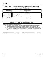
Step 8 - Plot the data. A more precise and refined picture comes into view once<br />
you plot your data (Viewgraph 12). You bring all of the previous steps together<br />
when you construct the graph.<br />
! The horizontal scale across the bottom of the graph contains the intervals that<br />
were calculated previously.<br />
! The vertical scale contains the count or frequency of observations within each<br />
of the intervals.<br />
! A bar is drawn <strong>for</strong> the height of each interval. The bars look like columns.<br />
! The height is determined by the number of observations or percentage of the<br />
total observations <strong>for</strong> each of the intervals.<br />
! The Histogram may not be perfectly symmetrical. Variations will occur. Ask<br />
yourself whether the picture is reasonable and logical, but be careful not to let<br />
your preconceived ideas influence your decisions unfairly.<br />
Step 9 - Add the title and legend. A title and a legend provide the who, what,<br />
when, where, and why (also illustrated in Viewgraph 12) that are important <strong>for</strong><br />
understanding and interpreting the data. This additional in<strong>for</strong>mation documents<br />
the nature of the data, where it came from, and when it was collected. The legend<br />
may include such things as the sample size, the dates and times involved, who<br />
collected the data, and identifiable equipment or work groups. It is important to<br />
include any in<strong>for</strong>mation that helps clarify what the data describes.<br />
14 HISTOGRAM
S<br />
H<br />
O<br />
T<br />
C<br />
O<br />
U<br />
N<br />
T<br />
LEGEND:<br />
25<br />
20<br />
15<br />
10<br />
5<br />
0<br />
<strong>Basic</strong> <strong>Tools</strong> <strong>for</strong> <strong>Process</strong> <strong>Improvement</strong><br />
How to Construct a Histogram<br />
Step 8 - Plot the data<br />
Step 9 - Add the title and legend<br />
MISS DISTANCE FOR MK 75 GUN TEST FIRING<br />
MISSES<br />
-180 -120 -060 000 060 120 180 240 300 360 420<br />
YARDS SHORT<br />
TARGET<br />
HITS<br />
YARDS LONG<br />
MISSES<br />
USS CROMMELIN (FFG-37), PACIFIC MISSILE FIRING RANGE, 135 BL&P ROUNDS/MOUNT 31, 25 JUNE 94<br />
HISTOGRAM VIEWGRAPH 12<br />
HISTOGRAM 15
<strong>Basic</strong> <strong>Tools</strong> <strong>for</strong> <strong>Process</strong> <strong>Improvement</strong><br />
How do we interpret a Histogram?<br />
A Histogram provides a visual representation so you can see where most of the<br />
measurements are located and how spread out they are. Your Histogram might<br />
show any of the following conditions (Viewgraph 13):<br />
! Most of the data were on target, with very little variation from it, as in<br />
Viewgraph 13A.<br />
! Although some data were on target, many others were dispersed away from<br />
the target, as in Viewgraph 13B.<br />
! Even when most of the data were close together, they were located off the<br />
target by a significant amount, as in Viewgraph 13C.<br />
! The data were off target and widely dispersed, as in Viewgraph 13D.<br />
This in<strong>for</strong>mation helps you see how well the process per<strong>for</strong>med and how consistent it<br />
was. You may be thinking, "So what? How will this help me do my job better?" Well,<br />
with the results of the process clearly depicted, we can find the answer to a vital<br />
question:<br />
Did the process produce goods and services which are within specification limits?<br />
Looking at the Histogram, you can see, not only whether you were within<br />
specification limits, but also how close to the target you were (Viewgraph 14).<br />
16 HISTOGRAM
Interpreting Histograms<br />
Location and Spread of Data<br />
A<br />
C<br />
<strong>Basic</strong> <strong>Tools</strong> <strong>for</strong> <strong>Process</strong> <strong>Improvement</strong><br />
Target Target<br />
Target Target<br />
HISTOGRAM VIEWGRAPH 13<br />
Interpreting Histograms<br />
Is <strong>Process</strong> Within Specification<br />
Limits?<br />
WITHIN LIMITS OUT OF SPEC<br />
LSL Target USL LSL Target USL<br />
LSL = Lower specification limit<br />
USL = Upper specification limit<br />
HISTOGRAM VIEWGRAPH 14<br />
HISTOGRAM 17<br />
B<br />
D
<strong>Basic</strong> <strong>Tools</strong> <strong>for</strong> <strong>Process</strong> <strong>Improvement</strong><br />
Portraying your data in a Histogram enables you to check rapidly on the number, or<br />
the percentage, of defects produced during the time you collected data. But unless<br />
you know whether the process was stable (Viewgraph 15), you won’t be able to<br />
predict whether future products will be within specification limits or determine a<br />
course of action to ensure that they are.<br />
A Histogram can show you whether or not your process is producing products or<br />
services that are within specification limits. To discover whether the process is<br />
stable, and to predict whether it can continue to produce within spec limits, you need<br />
to use a Control Chart (see the Control Chart module). Only after you have<br />
discovered whether your process is in or out of control can you determine an<br />
appropriate course of action—to eliminate special causes of variation, or to make<br />
fundamental changes to your process.<br />
There are times when a Histogram may look unusual to you. It might have more than<br />
one peak, be discontinued, or be skewed, with one tail longer than the other, as<br />
shown in Viewgraph 16. In these circumstances, the people involved in the process<br />
should ask themselves whether it really is unusual. The Histogram may not be<br />
symmetrical, but you may find out that it should look the way it does. On the other<br />
hand, the shape may show you that something is wrong, that data from several<br />
sources were mixed, <strong>for</strong> example, or different measurement devices were used, or<br />
operational definitions weren't applied. What is really important here is to avoid<br />
jumping to conclusions without properly examining the alternatives.<br />
18 HISTOGRAM
Target<br />
Interpreting Histograms<br />
<strong>Process</strong> Variation<br />
Day 1<br />
Target<br />
Day 2<br />
Day 3 Day 4<br />
Target<br />
Target<br />
HISTOGRAM VIEWGRAPH 15<br />
Skewed<br />
(not symmetrical)<br />
<strong>Basic</strong> <strong>Tools</strong> <strong>for</strong> <strong>Process</strong> <strong>Improvement</strong><br />
Interpreting Histograms<br />
Common Histogram Shapes<br />
Discontinued<br />
Symmetrical<br />
(mirror imaged)<br />
HISTOGRAM VIEWGRAPH 16<br />
HISTOGRAM 19
<strong>Basic</strong> <strong>Tools</strong> <strong>for</strong> <strong>Process</strong> <strong>Improvement</strong><br />
How can we practice what we've learned?<br />
Two exercises are provided that will take you through the nine steps <strong>for</strong> developing a<br />
Histogram. On the four pages that follow the scenario <strong>for</strong> Exercise 1 you will find a<br />
set of blank worksheets (Viewgraphs 17 through 23) to use in working through both<br />
of the exercises in this module.<br />
You will find a set of answer keys <strong>for</strong> Exercise 1 after the blank worksheets, and <strong>for</strong><br />
Exercise 2 after the description of its scenario. These answer keys represent only<br />
one possible set of answers. It's all right <strong>for</strong> you to choose an interval width or a<br />
number of intervals that is different from those used in the answer keys. Even<br />
though the shape of your Histogram may vary somewhat from the answer key's<br />
shape, it should be reasonably close unless you used a very different number of<br />
intervals.<br />
EXERCISE 1: The source of data <strong>for</strong> the first exercise is the following scenario. A<br />
list of the data collected follows this description. Use the blank worksheets in<br />
Viewgraphs 17 through 23 to do this exercise. You will find answer keys in<br />
Viewgraphs 24 through 30.<br />
Your corpsman is responsible <strong>for</strong> the semiannual Physical<br />
Readiness Test (PRT) screening <strong>for</strong> percent body fat. Prior<br />
to one PRT, the corpsman recorded the percent of body fat<br />
<strong>for</strong> the 80 personnel assigned to the command. These are<br />
the data collected:<br />
PERCENT BODY FAT RECORDED<br />
11 22 15 7 13 20 25 12 16 19<br />
4 14 11 16 18 32 10 16 17 10<br />
8 11 23 14 16 10 5 21 26 10<br />
23 12 10 16 17 24 11 20 9 13<br />
24 10 16 18 22 15 13 19 15 24<br />
11 20 15 13 9 18 22 16 18 9<br />
14 20 11 19 10 17 15 12 17 11<br />
17 11 15 11 15 16 12 28 14 13<br />
20 HISTOGRAM
<strong>Basic</strong> <strong>Tools</strong> <strong>for</strong> <strong>Process</strong> <strong>Improvement</strong><br />
WORKSHEET<br />
Step 1 - Count the number of data points<br />
TOTAL NUMBER =<br />
HISTOGRAM VIEWGRAPH 17<br />
WORKSHEET<br />
Step 2 - Summarize the data on a tally sheet<br />
VALUE TALLY VALUE TALLY VALUE TALLY VALUE TALLY VALUE TALLY<br />
HISTOGRAM VIEWGRAPH 18<br />
HISTOGRAM 21
<strong>Basic</strong> <strong>Tools</strong> <strong>for</strong> <strong>Process</strong> <strong>Improvement</strong><br />
WORKSHEET<br />
Step 3 - Compute the range <strong>for</strong> the data set<br />
Largest value = _______________<br />
Smallest value = _______________<br />
________________________________________<br />
Range of values = _______________<br />
HISTOGRAM VIEWGRAPH 19<br />
WORKSHEET<br />
Step 4 - Determine the number of intervals<br />
IF YOU HAVE THIS<br />
MANY DATA POINTS<br />
Less than 50<br />
50 to 99<br />
100 to 250<br />
More than 250<br />
USE THIS NUMBER<br />
OF INTERVALS:<br />
5 to 7 intervals<br />
6 to 10 intervals<br />
7 to 12 intervals<br />
10 to 20 intervals<br />
HISTOGRAM VIEWGRAPH 20<br />
22 HISTOGRAM
Interval<br />
Width<br />
<strong>Basic</strong> <strong>Tools</strong> <strong>for</strong> <strong>Process</strong> <strong>Improvement</strong><br />
WORKSHEET<br />
Step 5 - Compute the interval width<br />
=<br />
Range<br />
Number of<br />
Intervals<br />
= =<br />
Round up to<br />
next higher<br />
whole number<br />
HISTOGRAM VIEWGRAPH 21<br />
WORKSHEET<br />
Step 6 - Determine the starting point of each interval<br />
Step 7 - Count the number of points in each interval<br />
INTERVAL STARTING INTERVAL ENDING NUMBER<br />
NUMBER VALUE WIDTH VALUE OF COUNTS<br />
1<br />
2<br />
3<br />
4<br />
5<br />
6<br />
7<br />
8<br />
9<br />
10<br />
HISTOGRAM VIEWGRAPH 22<br />
HISTOGRAM 23
<strong>Basic</strong> <strong>Tools</strong> <strong>for</strong> <strong>Process</strong> <strong>Improvement</strong><br />
WORKSHEET<br />
Step 8 - Plot the data<br />
Step 9 - Add title and legend<br />
HISTOGRAM VIEWGRAPH 23<br />
24 HISTOGRAM
EXERCISE 1 ANSWER KEY<br />
Step 1 - Count the number of data points<br />
11 22 15 7 13 20 25 12 16 19<br />
4 14 11 16 18 32 10 16 17 10<br />
8 11 23 14 16 10 5 21 26 10<br />
23 12 10 16 17 24 11 20 9 13<br />
24 10 16 18 22 15 13 19 15 24<br />
11 20 15 13 9 18 22 16 18 9<br />
14 20 11 19 10 17 15 12 17 11<br />
17 11 15 11 15 16 12 28 14 13<br />
TOTAL = 80<br />
HISTOGRAM VIEWGRAPH 24<br />
EXERCISE 1 ANSWER KEY<br />
Step 2 - Summarize the data on a tally sheet<br />
%<br />
FAT NO. OF PERS<br />
0 0<br />
1 0<br />
2 0<br />
3 0<br />
4 1<br />
5 1<br />
6 0<br />
7 1<br />
8 1<br />
9 3<br />
10 7<br />
<strong>Basic</strong> <strong>Tools</strong> <strong>for</strong> <strong>Process</strong> <strong>Improvement</strong><br />
%<br />
FAT NO. OF PERS<br />
11 9<br />
12 4<br />
13 5<br />
14 4<br />
15 7<br />
16 8<br />
17 5<br />
18 4<br />
19 3<br />
20 4<br />
21 1<br />
%<br />
FAT NO. OF PERS<br />
22 3<br />
23 2<br />
24 3<br />
25 1<br />
26 1<br />
27 0<br />
28 1<br />
29 0<br />
30 0<br />
31 0<br />
32 1<br />
HISTOGRAM VIEWGRAPH 25<br />
HISTOGRAM 25
<strong>Basic</strong> <strong>Tools</strong> <strong>for</strong> <strong>Process</strong> <strong>Improvement</strong><br />
EXERCISE 1 ANSWER KEY<br />
Step 3 - Compute the range <strong>for</strong> the data set<br />
Largest value = 32 Percent body fat<br />
Smallest value = 4 Percent body fat<br />
_________________________________________<br />
Range of values = 28 Percent body fat<br />
HISTOGRAM VIEWGRAPH 26<br />
EXERCISE 1 ANSWER KEY<br />
Step 4 - Determine the number of intervals<br />
IF YOU HAVE THIS<br />
MANY DATA POINTS<br />
Less than 50<br />
50 to 99<br />
100 to 250<br />
More than 250<br />
USE THIS NUMBER<br />
OF INTERVALS:<br />
5 to 7 intervals<br />
6 to 10 intervals<br />
7 to 12 intervals<br />
10 to 20 intervals<br />
HISTOGRAM VIEWGRAPH 27<br />
26 HISTOGRAM
Interval<br />
Width<br />
<strong>Basic</strong> <strong>Tools</strong> <strong>for</strong> <strong>Process</strong> <strong>Improvement</strong><br />
Equal to or greater than<br />
the STARTING VALUE<br />
EXERCISE 1 ANSWER KEY<br />
Step 5 - Compute the interval width<br />
=<br />
Range<br />
Number of<br />
Intervals<br />
Use 8 <strong>for</strong> the number<br />
of intervals<br />
28<br />
= =<br />
8<br />
HISTOGRAM VIEWGRAPH 28<br />
EXERCISE 1 ANSWER KEY<br />
Step 6 - Determine the starting point of each interval<br />
Step 7 - Count the number of points in each interval<br />
INTERVAL STARTING INTERVAL ENDING NUMBER<br />
NUMBER VALUE WIDTH VALUE OF COUNTS<br />
1 4 + 4 8 3<br />
2 8 + 4 12 20<br />
3 12 + 4 16 20<br />
4 16 + 4 20 20<br />
5 20 + 4 24 10<br />
6 24 + 4 28 5<br />
7 28 + 4 32 1<br />
8 32 + 4 36 1<br />
But less than<br />
the ENDING VALUE<br />
HISTOGRAM VIEWGRAPH 29<br />
3.5<br />
Round up<br />
to 4<br />
HISTOGRAM 27
NO. OF PERSONNEL<br />
20<br />
18<br />
16<br />
14<br />
12<br />
10<br />
8<br />
6<br />
4<br />
2<br />
0<br />
<strong>Basic</strong> <strong>Tools</strong> <strong>for</strong> <strong>Process</strong> <strong>Improvement</strong><br />
0<br />
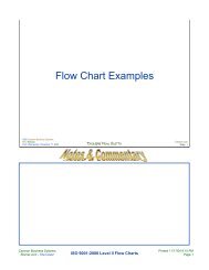
EXERCISE 1 ANSWER KEY<br />
Step 8 - Plot the data<br />
Step 9 - Add title and legend<br />
JUNE 94 PRT PERCENT BODY FAT<br />
SATISFACTORY % BODY FAT<br />
4 8 12 16 20 24 28 32 36<br />
PERCENT BODY FAT<br />
LEGEND: USS LEADER (MSO-490), 25 JUNE 94, ALL 80 PERSONNEL SAMPLED<br />
HISTOGRAM VIEWGRAPH 30<br />
28 HISTOGRAM
<strong>Basic</strong> <strong>Tools</strong> <strong>for</strong> <strong>Process</strong> <strong>Improvement</strong><br />
EXERCISE 2: The source of data <strong>for</strong> the second exercise is the following scenario.<br />
A listing of the data collected follows this description. Use the blank worksheets in<br />
Viewgraphs 17 through 23 to do this exercise. You will find answer keys in<br />
Viewgraphs 31 through 37.<br />
A Marine Corps small arms instructor was per<strong>for</strong>ming an<br />
analysis of 9 mm pistol marksmanship scores to improve<br />
training methods. For every class of 25, the instructor<br />
recorded the scores <strong>for</strong> each student who occupied the<br />
first four firing positions at the small arms range. The<br />
instructor then averaged the scores <strong>for</strong> each class,<br />
maintaining a database on 105 classes. These are the<br />
data collected:<br />
AVERAGE SMALL ARMS SCORES<br />
160 190 155 300 280 185 250 285 200 165<br />
175 190 210 225 275 240 170 185 215 220<br />
270 265 255 235 170 175 185 195 200 260<br />
180 245 270 200 200 220 265 270 250 230<br />
255 180 260 240 245 170 205 260 215 185<br />
255 245 210 225 225 235 230 230 195 225<br />
230 255 235 195 220 210 235 240 200 220<br />
195 235 230 215 225 235 225 200 245 230<br />
220 215 225 250 220 245 195 235 225 230<br />
210 240 215 230 220 225 200 235 215 240<br />
220 230 225 215 225<br />
HISTOGRAM 29
EXERCISE 2 ANSWER KEY<br />
Step 1 - Count the number of data points<br />
160 190 155 300 280 185 250 285 200 165<br />
175 190 210 225 275 240 170 185 215 220<br />
270 265 255 235 170 175 185 195 200 260<br />
180 245 270 200 200 220 265 270 250 230<br />
255 180 260 240 245 170 205 260 215 185<br />
255 245 210 225 225 235 230 230 195 225<br />
230 255 235 195 220 210 235 240 200 220<br />
195 235 230 215 225 235 225 200 245 230<br />
220 215 225 250 220 245 195 235 225 230<br />
210 240 215 230 220 225 200 235 215 240<br />
220 230 225 215 225<br />
TOTAL = 105<br />
HISTOGRAM VIEWGRAPH 31<br />
155 1<br />
160 1<br />
165 1<br />
170 3<br />
175 2<br />
180 2<br />
185 4<br />
190 2<br />
195 5<br />
200 7<br />
<strong>Basic</strong> <strong>Tools</strong> <strong>for</strong> <strong>Process</strong> <strong>Improvement</strong><br />
EXERCISE 2 ANSWER KEY<br />
Step 2 - Summarize the data on a tally sheet<br />
SCORE TALLY SCORE TALLY SCORE TALLY<br />
205 1<br />
210 4<br />
215 7<br />
220 8<br />
225 11<br />
230 9<br />
235 8<br />
240 5<br />
245 5<br />
250 3<br />
255 4<br />
260 3<br />
265 2<br />
270 3<br />
275 1<br />
280 1<br />
285 1<br />
290 0<br />
295 0<br />
300 1<br />
HISTOGRAM VIEWGRAPH 32<br />
30 HISTOGRAM
<strong>Basic</strong> <strong>Tools</strong> <strong>for</strong> <strong>Process</strong> <strong>Improvement</strong><br />
EXERCISE 2 ANSWER KEY<br />
Step 3 - Compute the range <strong>for</strong> the data set<br />
Largest value = 300 Points<br />
Smallest value = 155 Points<br />
__________________________________<br />
Range of values = 145 Points<br />
HISTOGRAM VIEWGRAPH 33<br />
EXERCISE 2 ANSWER KEY<br />
Step 4 - Determine the number of intervals<br />
IF YOU HAVE THIS<br />
MANY DATA POINTS<br />
Less than 50<br />
50 to 99<br />
100 to 250<br />
More than 250<br />
USE THIS NUMBER<br />
OF INTERVALS:<br />
5 to 7 intervals<br />
6 to 10 intervals<br />
7 to 12 intervals<br />
10 to 20 intervals<br />
HISTOGRAM VIEWGRAPH 34<br />
HISTOGRAM 31
Interval<br />
Width<br />
<strong>Basic</strong> <strong>Tools</strong> <strong>for</strong> <strong>Process</strong> <strong>Improvement</strong><br />
EXERCISE 2 ANSWER KEY<br />
Step 5 - Compute the interval width<br />
=<br />
HISTOGRAM VIEWGRAPH 35<br />
EXERCISE 2 ANSWER KEY<br />
Step 6 - Determine the starting point of each interval<br />
Step 7 - Count the number of points in each interval<br />
INTERVAL STARTING INTERVAL ENDING NUMBER<br />
NUMBER VALUE WIDTH VALUE OF COUNTS<br />
1 155 + 15 170 3<br />
2 170 + 15 185 7<br />
3 185 + 15 200 11<br />
4 200 + 15 215 12<br />
5 215 + 15 230 26<br />
6 230 + 15 245 22<br />
7 245 + 15 260 12<br />
8 260 + 15 275 8<br />
9 275 + 15 290 3<br />
10 290 + 15 300 1<br />
Equal to or greater than<br />
the STARTING VALUE<br />
Range<br />
Number of<br />
Intervals<br />
Use 10 <strong>for</strong> the number<br />
of intervals<br />
145<br />
= =<br />
10<br />
But less than<br />
the ENDING VALUE<br />
14.5<br />
Round up<br />
to 15<br />
HISTOGRAM VIEWGRAPH 36<br />
32 HISTOGRAM
NO. OF PERSONNEL<br />
30<br />
25<br />
20<br />
15<br />
10<br />
5<br />
0<br />
<strong>Basic</strong> <strong>Tools</strong> <strong>for</strong> <strong>Process</strong> <strong>Improvement</strong><br />
EXERCISE 2 ANSWER KEY<br />
Step 8 - Plot the data<br />
Step 9 - Add title and legend<br />
MARKSMANSHIP SCORES FOR 9mm PISTOL<br />
155 170 185 200 215 230 245 260 275 290 300<br />
SCORES<br />
LEGEND: MCBH KANEOHE BAY, HI; AVERAGE OF 4 SCORES PER CLASS, 105 CLASSES, 1 JUNE 94 - 15 JULY 94<br />
HISTOGRAM VIEWGRAPH 37<br />
HISTOGRAM 33
REFERENCES:<br />
<strong>Basic</strong> <strong>Tools</strong> <strong>for</strong> <strong>Process</strong> <strong>Improvement</strong><br />
1. Brassard, M. (1988). The Memory Jogger, A Pocket Guide of <strong>Tools</strong> <strong>for</strong><br />
Continuous <strong>Improvement</strong>, pp. 36 - 43. Methuen, MA: GOAL/QPC.<br />
2. Department of the Navy (November 1992), Fundamentals of Total Quality<br />
Leadership (Instructor Guide), pp. 6-44 - 6-47. San Diego, CA: Navy Personnel<br />
Research and Development Center.<br />
3. Department of the Navy (September 1993). Systems Approach to <strong>Process</strong><br />
<strong>Improvement</strong> (Instructor Guide), pp. 10-17 - 10-38. San Diego, CA: OUSN Total<br />
Quality Leadership Office and Navy Personnel Research and Development<br />
Center.<br />
4. Naval Medical Quality Institute (Undated). Total Quality Leader's Course (Student<br />
Guide), pp. U-26 - U-28. Bethesda, MD.<br />
34 HISTOGRAM
HISTOGRAM VIEWGRAPH 1<br />
• A bar graph that shows the distribution of data<br />
• A snapshot of data taken from a process<br />
0 5 10 15 20 25 30 35 40 45 50 55 60<br />
0<br />
20<br />
40<br />
60<br />
80<br />
100<br />
What Is a Histogram?
HISTOGRAM VIEWGRAPH 2<br />
• Assist in decision making<br />
• Communicate in<strong>for</strong>mation to the team<br />
• Compare measurements to specifications<br />
• Summarize large data sets graphically<br />
When Are Histograms Used?
HISTOGRAM VIEWGRAPH 3<br />
5<br />
1 Title 2 Horizontal / X-axis<br />
3 Bars 4 Vertical / Y-axis<br />
5 Legend<br />
MEAN TIME BETWEEN FAILURE (IN DAYS) FOR R-1051 HF RECEIVER<br />
Data taken at SIMA, Pearl Harbor, 15 May - 15 July 94<br />
0 5 10 15 20 25 30 35 40 45 50 55 60<br />
DAYS OF OPERATION<br />
2<br />
0<br />
F<br />
R<br />
E<br />
Q<br />
U<br />
E<br />
N<br />
C<br />
Y<br />
20<br />
4<br />
40<br />
3<br />
60<br />
80<br />
100<br />
DAYS OF OPERATION PRIOR TO<br />
FAILURE FOR AN HF RECEIVER<br />
1<br />
Parts of a Histogram
HISTOGRAM VIEWGRAPH 4<br />
Step 5 - Compute interval width<br />
Step 4 - Determine number of intervals<br />
Step 3 - Compute the range<br />
Step 2 - Summarize on a tally sheet<br />
Step 1 - Count number of data points<br />
Constructing a Histogram
HISTOGRAM VIEWGRAPH 5<br />
Step 9 - Add title and legend<br />
Step 8 - Plot the data<br />
Step 7 - Count number of points in<br />
each interval<br />
Step 6 - Determine interval starting<br />
points<br />
Constructing a Histogram
HISTOGRAM VIEWGRAPH 6<br />
-180 30 190 380 330 140 160 270 10 - 90<br />
- 10 30 60 230 90 120 10 50 250 180<br />
-130 220 170 130 - 50 - 80 180 100 110 200<br />
260 190 -100 150 210 140 -130 130 150 370<br />
160 180 240 260 - 20 - 80 30 80 240 130<br />
210 40 70 - 70 250 360 120 - 60 - 30 200<br />
50 20 30 280 410 70 - 10 20 130 170<br />
140 220 - 40 290 90 100 - 30 340 20 80<br />
210 130 350 250 - 20 230 180 130 - 30 210<br />
-30 80 270 320 30 240 120 100 20 70<br />
300 260 20 40 - 20 250 310 40 200 190<br />
110 -30 50 240 180 50 130 200 280 60<br />
260 70 100 140 80 190 100 270 140 80<br />
110 130 120 30 70<br />
TOTAL = 135<br />
Number of yards long (+ data) and yards short (- data) that a gun crew missed its target.<br />
Step 1 - Count the total number of data points<br />
How to Construct a Histogram
HISTOGRAM VIEWGRAPH 7<br />
410<br />
1<br />
- 180 1 - 20 3 90 2 190 4 290 1<br />
- 130 2 - 10 2 100 5 200 4 300 1<br />
- 100 1 10 2 110 3 210 4 310 1<br />
- 90 1 20 5 120 4 220 2 320 1<br />
- 80 2 30 6 130 8 230 2 330 1<br />
- 70 1 40 3 140 5 240 4 340 1<br />
- 60 1 50 4 150 2 250 4 350 1<br />
- 50 1 60 2 160 2 260 4 360 1<br />
- 40 1 70 5 170 2 270 3 370 1<br />
- 30 5 80 5 180 5 280 2 380 1<br />
DATA TALLY DATA TALLY DATA TALLY DATA TALLY DATA TALLY<br />
Step 2 - Summarize the data on a tally sheet<br />
How to Construct a Histogram
HISTOGRAM VIEWGRAPH 8<br />
Calculation: + 410 - (- 180) = 410 + 180 = 590<br />
Range of values = 590 yards<br />
Smallest value = - 180 yards short of target<br />
Largest value = + 410 yards past target<br />
Step 3 - Compute the range <strong>for</strong> the data set<br />
How to Construct a Histogram
HISTOGRAM VIEWGRAPH 9<br />
More than 250<br />
10 to 20 intervals<br />
100 to 250<br />
7 to 12 intervals<br />
50 to 99<br />
6 to 10 intervals<br />
Less than 50<br />
5 to 7 intervals<br />
IF YOU HAVE THIS<br />
MANY DATA POINTS<br />
USE THIS NUMBER<br />
OF INTERVALS:<br />
Step 4 - Determine the number of intervals<br />
required<br />
How to Construct a Histogram
HISTOGRAM VIEWGRAPH 10<br />
Round up<br />
to 60<br />
Use Use 10 10 <strong>for</strong> <strong>for</strong> the the<br />
number of of intervals<br />
Number of<br />
Intervals<br />
Interval<br />
Width<br />
10<br />
=<br />
=<br />
=<br />
59<br />
Range<br />
590<br />
Step 5 - Compute the interval width<br />
How to Construct a Histogram
HISTOGRAM VIEWGRAPH 11<br />
Equal to or greater than the<br />
STARTING VALUE<br />
But less than the<br />
ENDING VALUE<br />
10<br />
360<br />
60<br />
420<br />
4<br />
9<br />
300<br />
60<br />
360<br />
6<br />
8<br />
240<br />
60<br />
300<br />
18<br />
7<br />
180<br />
60<br />
240<br />
20<br />
6<br />
120<br />
60<br />
180<br />
24<br />
5<br />
060<br />
60<br />
120<br />
22<br />
4<br />
000<br />
60<br />
060<br />
20<br />
3<br />
-060<br />
60<br />
000<br />
13<br />
2<br />
-120<br />
60<br />
-060<br />
5<br />
1<br />
-180<br />
60<br />
-120<br />
3<br />
INTERVAL<br />
NUMBER<br />
STARTING<br />
VALUE<br />
INTERVAL<br />
WIDTH<br />
ENDING<br />
VALUE<br />
NUMBER OF<br />
COUNTS<br />
Step 7 - Count the number of points in each interval<br />
Step 6 - Determine the starting point of each interval<br />
How to Construct a Histogram
HISTOGRAM VIEWGRAPH 12<br />
LEGEND:<br />
USS CROMMELIN (FFG-37), PACIFIC MISSILE FIRING RANGE, 135 BL&P ROUNDS/MOUNT 31, 25 JUNE 94<br />
TARGET<br />
YARDS SHORT<br />
YARDS LONG<br />
-180 -120 -060 000 060 120 180 240 300 360 420<br />
0<br />
C<br />
O<br />
U<br />
N<br />
T<br />
5<br />
10<br />
15<br />
S<br />
H<br />
O<br />
T<br />
20<br />
25<br />
MISSES<br />
MISSES<br />
HITS<br />
MISS DISTANCE FOR MK 75 GUN TEST FIRING<br />
Step 8 - Plot the data<br />
Step 9 - Add the title and legend<br />
How to Construct a Histogram
HISTOGRAM VIEWGRAPH 13<br />
Target Target<br />
C<br />
D<br />
Target Target<br />
A<br />
B<br />
Interpreting Histograms<br />
Location and Spread of Data
HISTOGRAM VIEWGRAPH 14<br />
LSL = Lower specification limit<br />
USL = Upper specification limit<br />
LSL Target USL LSL Target USL<br />
WITHIN LIMITS OUT OF SPEC<br />
Interpreting Histograms<br />
Is <strong>Process</strong> Within Specification<br />
Limits?
HISTOGRAM VIEWGRAPH 15<br />
Target<br />
Target<br />
Day 3 Day 4<br />
Target<br />
Target<br />
Day 1<br />
Day 2<br />
Interpreting Histograms<br />
<strong>Process</strong> Variation
HISTOGRAM VIEWGRAPH 16<br />
Symmetrical<br />
(mirror imaged)<br />
Discontinued<br />
Skewed<br />
(not symmetrical)<br />
Interpreting Histograms<br />
Common Histogram Shapes
HISTOGRAM VIEWGRAPH 17<br />
TOTAL NUMBER =<br />
Step 1 - Count the number of data points<br />
WORKSHEET
HISTOGRAM VIEWGRAPH 18<br />
VALUE TALLY VALUE TALLY VALUE TALLY VALUE TALLY VALUE TALLY<br />
Step 2 - Summarize the data on a tally sheet<br />
WORKSHEET
HISTOGRAM VIEWGRAPH 19<br />
Range of values = _______________<br />
________________________________________<br />
Smallest value = _______________<br />
Largest value = _______________<br />
Step 3 - Compute the range <strong>for</strong> the data set<br />
WORKSHEET
HISTOGRAM VIEWGRAPH 20<br />
More than 250<br />
10 to 20 intervals<br />
100 to 250<br />
7 to 12 intervals<br />
50 to 99<br />
6 to 10 intervals<br />
Less than 50<br />
5 to 7 intervals<br />
IF YOU HAVE THIS<br />
MANY DATA POINTS<br />
USE THIS NUMBER<br />
OF INTERVALS:<br />
Step 4 - Determine the number of intervals<br />
WORKSHEET
HISTOGRAM VIEWGRAPH 21<br />
Round up to<br />
next higher<br />
whole number<br />
Number of<br />
Intervals<br />
Interval<br />
Width<br />
=<br />
= =<br />
Range<br />
Step 5 - Compute the interval width<br />
WORKSHEET
HISTOGRAM VIEWGRAPH 22<br />
INTERVAL STARTING INTERVAL ENDING NUMBER<br />
NUMBER VALUE WIDTH VALUE OF COUNTS<br />
1<br />
2<br />
3<br />
4<br />
5<br />
6<br />
7<br />
8<br />
9<br />
10<br />
Step 7 - Count the number of points in each interval<br />
Step 6 - Determine the starting point of each interval<br />
WORKSHEET
HISTOGRAM VIEWGRAPH 23<br />
Step 8 - Plot the data<br />
Step 9 - Add title and legend<br />
WORKSHEET
HISTOGRAM VIEWGRAPH 24<br />
TOTAL = 80<br />
17 11 15 11 15 16 12 28 14 13<br />
14 20 11 19 10 17 15 12 17 11<br />
11 20 15 13 9 18 22 16 18 9<br />
24 10 16 18 22 15 13 19 15 24<br />
23 12 10 16 17 24 11 20 9 13<br />
8 11 23 14 16 10 5 21 26 10<br />
4 14 11 16 18 32 10 16 17 10<br />
11 22 15 7 13 20 25 12 16 19<br />
Step 1 - Count the number of data points<br />
EXERCISE 1 ANSWER KEY
HISTOGRAM VIEWGRAPH 25<br />
%<br />
FAT NO. OF PERS<br />
0 0<br />
1 0<br />
2 0<br />
3 0<br />
4 1<br />
5 1<br />
6 0<br />
7 1<br />
8 1<br />
9 3<br />
10 7<br />
%<br />
FAT NO. OF PERS<br />
11 9<br />
12 4<br />
13 5<br />
14 4<br />
15 7<br />
16 8<br />
17 5<br />
18 4<br />
19 3<br />
20 4<br />
21 1<br />
%<br />
FAT NO. OF PERS<br />
22 3<br />
23 2<br />
24 3<br />
25 1<br />
26 1<br />
27 0<br />
28 1<br />
29 0<br />
30 0<br />
31 0<br />
32 1<br />
Step 2 - Summarize the data on a tally sheet<br />
EXERCISE 1 ANSWER KEY
HISTOGRAM VIEWGRAPH 26<br />
Range of values = 28 Percent body fat<br />
_________________________________________<br />
Smallest value = 4 Percent body fat<br />
Largest value = 32 Percent body fat<br />
Step 3 - Compute the range <strong>for</strong> the data set<br />
EXERCISE 1 ANSWER KEY
HISTOGRAM VIEWGRAPH 27<br />
More than 250<br />
10 to 20 intervals<br />
100 to 250<br />
7 to 12 intervals<br />
50 to 99<br />
6 to 10 intervals<br />
Less than 50<br />
5 to 7 intervals<br />
IF YOU HAVE THIS<br />
MANY DATA POINTS<br />
USE THIS NUMBER<br />
OF INTERVALS:<br />
Step 4 - Determine the number of intervals<br />
EXERCISE 1 ANSWER KEY
HISTOGRAM VIEWGRAPH 28<br />
Round up<br />
to 4<br />
Use 8 <strong>for</strong> the number<br />
of intervals<br />
Number of<br />
Intervals<br />
Interval<br />
Width<br />
=<br />
3.5<br />
Range<br />
28<br />
= =<br />
8<br />
Step 5 - Compute the interval width<br />
EXERCISE 1 ANSWER KEY
HISTOGRAM VIEWGRAPH 29<br />
Equal to or greater than<br />
the STARTING VALUE<br />
But less than<br />
the ENDING VALUE<br />
7 28 + 4 32 1<br />
8 32 + 4 36 1<br />
5 20 + 4 24 10<br />
6 24 + 4 28 5<br />
3 12 + 4 16 20<br />
4 16 + 4 20 20<br />
1 4 + 4 8 3<br />
2 8 + 4 12 20<br />
INTERVAL STARTING INTERVAL ENDING NUMBER<br />
NUMBER VALUE WIDTH VALUE OF COUNTS<br />
Step 7 - Count the number of points in each interval<br />
Step 6 - Determine the starting point of each interval<br />
EXERCISE 1 ANSWER KEY
HISTOGRAM VIEWGRAPH 30<br />
LEGEND: USS LEADER (MSO-490), 25 JUNE 94, ALL 80 PERSONNEL SAMPLED<br />
0<br />
4 8 12 16 20 24 28 32 36<br />
PERCENT BODY FAT<br />
0<br />
2<br />
4<br />
NO. OF PERSONNEL<br />
6<br />
8<br />
10<br />
12<br />
14<br />
16<br />
18<br />
20<br />
SATISFACTORY % BODY FAT<br />
JUNE 94 PRT PERCENT BODY FAT<br />
Step 8 - Plot the data<br />
Step 9 - Add title and legend<br />
EXERCISE 1 ANSWER KEY
HISTOGRAM VIEWGRAPH 31<br />
TOTAL = 105<br />
220 230 225 215 225<br />
210 240 215 230 220 225 200 235 215 240<br />
220 215 225 250 220 245 195 235 225 230<br />
195 235 230 215 225 235 225 200 245 230<br />
230 255 235 195 220 210 235 240 200 220<br />
255 245 210 225 225 235 230 230 195 225<br />
255 180 260 240 245 170 205 260 215 185<br />
180 245 270 200 200 220 265 270 250 230<br />
270 265 255 235 170 175 185 195 200 260<br />
175 190 210 225 275 240 170 185 215 220<br />
160 190 155 300 280 185 250 285 200 165<br />
Step 1 - Count the number of data points<br />
EXERCISE 2 ANSWER KEY
HISTOGRAM VIEWGRAPH 32<br />
200 7<br />
250 3<br />
300 1<br />
195 5<br />
245 5<br />
295 0<br />
190 2<br />
240 5<br />
290 0<br />
185 4<br />
235 8<br />
285 1<br />
180 2<br />
230 9<br />
280 1<br />
175 2<br />
225 11<br />
275 1<br />
170 3<br />
220 8<br />
270 3<br />
165 1<br />
215 7<br />
265 2<br />
160 1<br />
210 4<br />
260 3<br />
155 1<br />
205 1<br />
255 4<br />
SCORE TALLY SCORE TALLY SCORE TALLY<br />
Step 2 - Summarize the data on a tally sheet<br />
EXERCISE 2 ANSWER KEY
HISTOGRAM VIEWGRAPH 33<br />
Range of values = 145 Points<br />
__________________________________<br />
Smallest value = 155 Points<br />
Largest value = 300 Points<br />
Step 3 - Compute the range <strong>for</strong> the data set<br />
EXERCISE 2 ANSWER KEY
HISTOGRAM VIEWGRAPH 34<br />
More than 250<br />
10 to 20 intervals<br />
100 to 250<br />
7 to 12 intervals<br />
50 to 99<br />
6 to 10 intervals<br />
Less than 50<br />
5 to 7 intervals<br />
IF YOU HAVE THIS<br />
MANY DATA POINTS<br />
USE THIS NUMBER<br />
OF INTERVALS:<br />
Step 4 - Determine the number of intervals<br />
EXERCISE 2 ANSWER KEY
HISTOGRAM VIEWGRAPH 35<br />
Round up<br />
to 15<br />
Use 10 <strong>for</strong> the number<br />
of intervals<br />
Number of<br />
Intervals<br />
Interval<br />
Width<br />
=<br />
14.5<br />
Range<br />
145<br />
= =<br />
10<br />
Step 5 - Compute the interval width<br />
EXERCISE 2 ANSWER KEY
HISTOGRAM VIEWGRAPH 36<br />
Equal to or greater than<br />
the STARTING VALUE<br />
But less than<br />
the ENDING VALUE<br />
1 155 + 15 170 3<br />
2 170 + 15 185 7<br />
3 185 + 15 200 11<br />
4 200 + 15 215 12<br />
5 215 + 15 230 26<br />
6 230 + 15 245 22<br />
7 245 + 15 260 12<br />
8 260 + 15 275 8<br />
9 275 + 15 290 3<br />
10 290 + 15 300 1<br />
INTERVAL STARTING INTERVAL ENDING NUMBER<br />
NUMBER VALUE WIDTH VALUE OF COUNTS<br />
Step 7 - Count the number of points in each interval<br />
Step 6 - Determine the starting point of each interval<br />
EXERCISE 2 ANSWER KEY
HISTOGRAM VIEWGRAPH 37<br />
LEGEND: MCBH KANEOHE BAY, HI; AVERAGE OF 4 SCORES PER CLASS, 105 CLASSES, 1 JUNE 94 - 15 JULY 94<br />
SCORES<br />
155 170 185 200 215 230 245 260 275 290 300<br />
NO. OF PERSONNEL<br />
30<br />
25<br />
20<br />
15<br />
10<br />
5<br />
0<br />
MARKSMANSHIP SCORES FOR 9mm PISTOL<br />
Step 9 - Add title and legend<br />
Step 8 - Plot the data<br />
EXERCISE 2 ANSWER KEY