Wall Pressure and Shear Stress Spectra from Direct Numerical ...

2 HU, MORFEY, AND SANDHAM
@u i
@t
ijku j! k 1i
@
@x i
1
Re
@ 2 u i
@x j@x j
where the Reynolds number is Re u h = , with being the
kinematic viscosity. p uiui=2 is the modified pressure, ijk is
the permutation tensor, and ! k ijk@uj=@xi is the vorticity.
Poiseuille flow is driven by a mean pressure gradient, whose
nondimensional value is equal to 1. The channel coordinates are
x1 x in the streamwise direction, x2 y in the spanwise direction,
and x 3
(2)
z in the wall-normal direction, with the channel walls at
z 1. u; v; w denote the nondimensional velocities in the
x; y; z directions.
The spectral method of Kleiser and Schumann [17] has been used
to solve the incompressible governing equations with Fourier
discretization applied to the two periodic directions x; y , and
Chebyshev polynomial expansion to the wall-normal direction z.In
the periodic directions a twofold discrete Fourier transformation is
carried out for any quantity q by the following forward and backward
transforms:
~q k xl;k ym
1
XN y 1
Ny j 0
exp ik ymy j
q x i;y j ~q 0;y j 2 XN x=2
1
XN x 1
Nx i 0
l 1
XN y=2
m N y=2
q x i;y j exp ik xlx i
~q k xl;k ym exp ik ymy j
exp ikxlxi (4)
p
where i 1.
kxl 2 l=Lx 0 l Nx=2 and kym 2 m=
Ly Ny=2 m Ny=2 are wave numbers in the x and y
directions, respectively. The grid coordinates are uniform in the
streamwise and spanwise directions with xi iLx=Nx 0 i Nx and yj jLy=Ny 0 j Ny , and are stretched in the wall-normal
Q1 direction with zk cos k= Nz 1 0 k Nz 1 .(Nx Ny Nz) grid points are used in the computational box of size Lx Ly 2.
Time advance is achieved with a third-order Runge–Kutta method
for the convective term and the Crank–Nicolson method for the
pressure and viscous terms. An implicit treatment is employed to
avoid extremely small time steps in the near wall region resulting
from the Chebyshev discretization. De-aliasing via the “3=2 rule” has
been applied to the nonlinear convective term. More details on the
method can be found in [14,15,18,19].
B. DNS Cases and Results
Simulations have been carried out for turbulent channel flow at a
series of Reynolds numbers up to Re 1440. Large boxes have
been used for each case to include the large scale structures in the
computational domain. This is checked by making sure that the twopoint
correlation functions for velocity and pressure drop to zero at
large separation [14,15]. In the x and y directions, resolutions are
kept the same in wall units for all calculations, at x 16:88 and
y 8:44 (the Re 130 case has slightly lower values); these
values are comparable to those used by KMM [9]. In the wall-normal
direction more than 10 points are located in the near wall region
(3)
z < 9, with the first point 0.12 to 0.03 wall units from the wall. The
grid spacing at the channel centerline increases from 4.71 wall units
for Re 90 to 9.42 for Re 1440. For higher Reynolds number
cases, it is comparable to y but still lower than x .
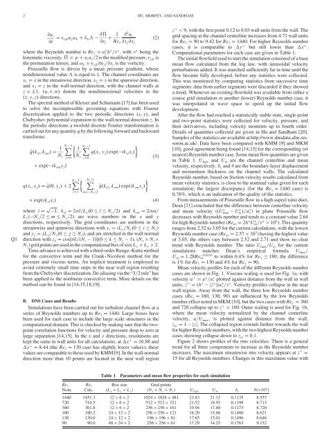
Computational parameters for each case are given in Table 1.
The initial flowfield used to start the simulation consisted of a base
mean flow calculated from the log law, with sinusoidal velocity
perturbations added. It was marched sufficiently far in time until the
flow became fully developed, before any statistics were collected.
This was monitored by comparing statistics from successive time
segments; data from earlier segments were discarded if they showed
a trend. Whenever an existing flowfield was available from either a
coarse grid simulation or another (lower) Reynolds number case, it
was interpolated in wave space to speed up the initial flow
development.
After the flow had reached a statistically stable state, single-point
and two-point statistics were collected for velocity, pressure, and
their derivatives, including velocity moments up to fourth order.
Details of quantities collected are given in Hu and Sandham [20].
Samples of the statistics are available at http://www.dnsdata.afm.ses.
soton.ac.uk/. Data have been compared with KMM [9] and MKM
[10], good agreement being found [14,15] for the corresponding (or
nearest) Reynolds number case. Some mean flow quantities are given
in Table 1. Umax and Um are the channel centerline and mean
velocity, respectively. 1 and are the boundary-layer displacement
and momentum thickness on the channel walls. The calculated
Reynolds number, based on friction velocity results calculated from
mean velocity statistics, is close to the nominal value given for each
simulation; the largest discrepancy (for the Re 1440 case) is
0.78%, which is an indication of the quality of the statistics.
From measurements of Poiseuille flow in a high aspect ratio duct,
Dean [21] concluded that the difference between centerline velocity
and mean velocity ( U max
U m =u ) in plane Poiseuille flow
decreases with Reynolds number and tends to a constant value 2.64
for high Reynolds number (Re m 2h U m= > 10 5 ). This quantity
ranges from 2.52 to 3.05 for the current calculations, with the lowest
Reynolds number case (Re m 2:57 10 3 ) having the highest value
of 3.05; the others vary between 2.52 and 2.71 and show no clear
trend with Reynolds number. The ratio U max=U m for the current
simulations matches Dean’s empirical formula U max=
Um 1:28Re 0:0116
m to within 0.4% for Re
is 1% for Re 130 and 4% for Re 90.
180; the difference
Mean velocity profiles for each of the different Reynolds number
cases are shown in Fig. 1. Viscous scaling is used for Fig. 1a, with
velocity u u =u plotted against distance from the wall in wall
units, z h jz j u = . Velocity profiles collapse in the near
wall region. Away from the wall, the three low Reynolds number
cases (Re 180, 130, 90) are influenced by the low Reynolds
number effect noted in MKM [10], but the two cases with Re 360
and 720 collapse up to z 100. Outer scaling is used for Fig. 1b,
where the mean velocity normalized by the channel centerline
velocity, u=Umax, is plotted against distance from the wall,
zw 1 jzj. The collapsed region extends further towards the wall
for higher Reynolds numbers, with the two highest Reynolds number
cases showing collapse down to z w
Table 1 Parameters and mean flow properties for each simulation
0:1.
Figure 2 shows profiles of the rms velocities. There is a general
trend for all three components to increase as the Reynolds number
increases. The maximum streamwise rms velocity appears at z
15 for all Reynolds numbers. Changes in this maximum value with
Re Re Box size Grid points
Nom. Calc. (Lx Ly Lz) (NxNyNz) Umax Um 1 102 1440 1451.3 12 6 2 1024 1024 481 23.83 21.12 0.1135 8.557
720 716.5 12 6 2 512 512 321 21.52 18.93 0.1198 8.713
360 361.8 12 6 2 256 256 161 19.94 17.40 0.1273 8.720
180 180.2 24 12 2 256 256 121 18.20 15.66 0.1400 8.621
130 130.0 24 12 2 196 196 81 17.65 15.01 0.1496 8.646
90 90.0 48 24 2 256 256 61 17.29 14.25 0.1763 9.152