Wall Pressure and Shear Stress Spectra from Direct Numerical ...

AIAA JOURNAL
Wall Pressure and Shear Stress Spectra
from Direct Numerical Simulations
of Channel Flow up to Re 1440
Z. W. Hu, ∗ C. L. Morfey, † and N. D. Sandham ‡
University of Southampton, Southampton, SO17 1BJ England, United Kingdom
DOI: 10.2514/1.17638
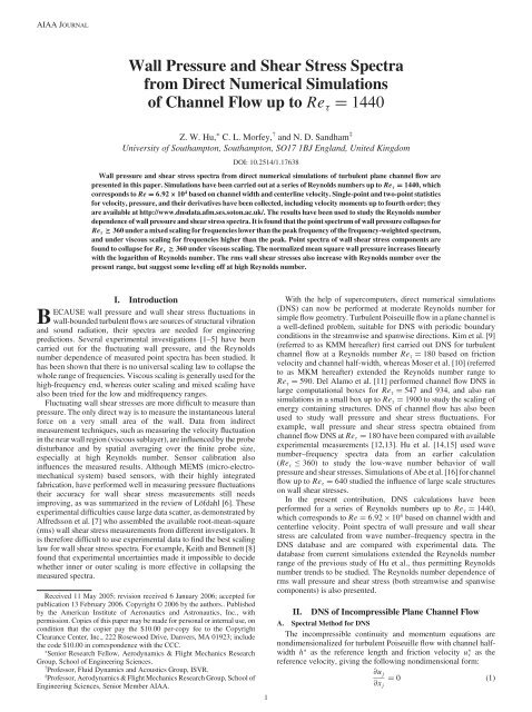
Wall pressure and shear stress spectra from direct numerical simulations of turbulent plane channel flow are
presented in this paper. Simulations have been carried out at a series of Reynolds numbers up to Re 1440, which
corresponds to Re 6:92 104 based on channel width and centerline velocity. Single-point and two-point statistics
for velocity, pressure, and their derivatives have been collected, including velocity moments up to fourth order; they
are available at http://www.dnsdata.afm.ses.soton.ac.uk/. The results have been used to study the Reynolds number
dependence of wall pressure and shear stress spectra. It is found that the point spectrum of wall pressure collapses for
Re 360 under a mixed scaling for frequencies lower than the peak frequency of the frequency-weighted spectrum,
and under viscous scaling for frequencies higher than the peak. Point spectra of wall shear stress components are
found to collapse for Re 360 under viscous scaling. The normalized mean square wall pressure increases linearly
with the logarithm of Reynolds number. The rms wall shear stresses also increase with Reynolds number over the
present range, but suggest some leveling off at high Reynolds number.
I. Introduction
BECAUSE wall pressure and wall shear stress fluctuations in
wall-bounded turbulent flows are sources of structural vibration
and sound radiation, their spectra are needed for engineering
predictions. Several experimental investigations [1–5] have been
carried out for the fluctuating wall pressure, and the Reynolds
number dependence of measured point spectra has been studied. It
has been shown that there is no universal scaling law to collapse the
whole range of frequencies. Viscous scaling is generally used for the
high-frequency end, whereas outer scaling and mixed scaling have
also been tried for the low and midfrequency ranges.
Fluctuating wall shear stresses are more difficult to measure than
pressure. The only direct way is to measure the instantaneous lateral
force on a very small area of the wall. Data from indirect
measurement techniques, such as measuring the velocity fluctuation
in the near wall region (viscous sublayer), are influenced by the probe
disturbance and by spatial averaging over the finite probe size,
especially at high Reynolds number. Sensor calibration also
influences the measured results. Although MEMS (micro-electromechanical
system) based sensors, with their highly integrated
fabrication, have performed well in measuring pressure fluctuations
their accuracy for wall shear stress measurements still needs
improving, as was summarized in the review of Löfdahl [6]. These
experimental difficulties cause large data scatter, as demonstrated by
Alfredsson et al. [7] who assembled the available root-mean-square
(rms) wall shear stress measurements from different investigators. It
is therefore difficult to use experimental data to find the best scaling
law for wall shear stress spectra. For example, Keith and Bennett [8]
found that experimental uncertainties made it impossible to decide
whether inner or outer scaling is more effective in collapsing the
measured spectra.
Received 11 May 2005; revision received 6 January 2006; accepted for
publication 13 February 2006. Copyright © 2006 by the authors.. Published
by the American Institute of Aeronautics and Astronautics, Inc., with
permission. Copies of this paper may be made for personal or internal use, on
condition that the copier pay the $10.00 per-copy fee to the Copyright
Clearance Center, Inc., 222 Rosewood Drive, Danvers, MA 01923; include
the code $10.00 in correspondence with the CCC.
∗ Senior Research Fellow, Aerodynamics & Flight Mechanics Research
Group, School of Engineering Sciences.
† Professor, Fluid Dynamics and Acoustics Group, ISVR.
‡ Professor, Aerodynamics & Flight Mechanics Research Group, School of
Engineering Sciences, Senior Member AIAA.
1
With the help of supercomputers, direct numerical simulations
(DNS) can now be performed at moderate Reynolds number for
simple flow geometry. Turbulent Poiseuille flow in a plane channel is
a well-defined problem, suitable for DNS with periodic boundary
conditions in the streamwise and spanwise directions. Kim et al. [9]
(referred to as KMM hereafter) first carried out DNS for turbulent
channel flow at a Reynolds number Re 180 based on friction
velocity and channel half-width, whereas Moser et al. [10] (referred
to as MKM hereafter) extended the Reynolds number range to
Re 590. Del Alamo et al. [11] performed channel flow DNS in
large computational boxes for Re 547 and 934, and also ran
simulations in a small box up to Re 1900 to study the scaling of
energy containing structures. DNS of channel flow has also been
used to study wall pressure and shear stress fluctuations. For
example, wall pressure and shear stress spectra obtained from
channel flow DNS at Re 180 have been compared with available
experimental measurements [12,13]. Hu et al. [14,15] used wave
number–frequency spectra data from an earlier calculation
(Re 360) to study the low-wave number behavior of wall
pressure and shear stresses. Simulations of Abe et al. [16] for channel
flow up to Re 640 studied the influence of large scale structures
on wall shear stresses.
In the present contribution, DNS calculations have been
performed for a series of Reynolds numbers up to Re 1440,
which corresponds to Re 6:92 10 4 based on channel width and
centerline velocity. Point spectra of wall pressure and wall shear
stress are calculated from wave number–frequency spectra in the
DNS database and are compared with experimental data. The
database from current simulations extended the Reynolds number
range of the previous study of Hu et al., thus permitting Reynolds
number trends to be studied. The Reynolds number dependence of
rms wall pressure and shear stress (both streamwise and spanwise
components) is also presented.
II. DNS of Incompressible Plane Channel Flow
A. Spectral Method for DNS
The incompressible continuity and momentum equations are
nondimensionalized for turbulent Poiseuille flow with channel halfwidth
h as the reference length and friction velocity u as the
reference velocity, giving the following nondimensional form:
@uj @xj 0 (1)

2 HU, MORFEY, AND SANDHAM
@u i
@t
ijku j! k 1i
@
@x i
1
Re
@ 2 u i
@x j@x j
where the Reynolds number is Re u h = , with being the
kinematic viscosity. p uiui=2 is the modified pressure, ijk is
the permutation tensor, and ! k ijk@uj=@xi is the vorticity.
Poiseuille flow is driven by a mean pressure gradient, whose
nondimensional value is equal to 1. The channel coordinates are
x1 x in the streamwise direction, x2 y in the spanwise direction,
and x 3
(2)
z in the wall-normal direction, with the channel walls at
z 1. u; v; w denote the nondimensional velocities in the
x; y; z directions.
The spectral method of Kleiser and Schumann [17] has been used
to solve the incompressible governing equations with Fourier
discretization applied to the two periodic directions x; y , and
Chebyshev polynomial expansion to the wall-normal direction z.In
the periodic directions a twofold discrete Fourier transformation is
carried out for any quantity q by the following forward and backward
transforms:
~q k xl;k ym
1
XN y 1
Ny j 0
exp ik ymy j
q x i;y j ~q 0;y j 2 XN x=2
1
XN x 1
Nx i 0
l 1
XN y=2
m N y=2
q x i;y j exp ik xlx i
~q k xl;k ym exp ik ymy j
exp ikxlxi (4)
p
where i 1.
kxl 2 l=Lx 0 l Nx=2 and kym 2 m=
Ly Ny=2 m Ny=2 are wave numbers in the x and y
directions, respectively. The grid coordinates are uniform in the
streamwise and spanwise directions with xi iLx=Nx 0 i Nx and yj jLy=Ny 0 j Ny , and are stretched in the wall-normal
Q1 direction with zk cos k= Nz 1 0 k Nz 1 .(Nx Ny Nz) grid points are used in the computational box of size Lx Ly 2.
Time advance is achieved with a third-order Runge–Kutta method
for the convective term and the Crank–Nicolson method for the
pressure and viscous terms. An implicit treatment is employed to
avoid extremely small time steps in the near wall region resulting
from the Chebyshev discretization. De-aliasing via the “3=2 rule” has
been applied to the nonlinear convective term. More details on the
method can be found in [14,15,18,19].
B. DNS Cases and Results
Simulations have been carried out for turbulent channel flow at a
series of Reynolds numbers up to Re 1440. Large boxes have
been used for each case to include the large scale structures in the
computational domain. This is checked by making sure that the twopoint
correlation functions for velocity and pressure drop to zero at
large separation [14,15]. In the x and y directions, resolutions are
kept the same in wall units for all calculations, at x 16:88 and
y 8:44 (the Re 130 case has slightly lower values); these
values are comparable to those used by KMM [9]. In the wall-normal
direction more than 10 points are located in the near wall region
(3)
z < 9, with the first point 0.12 to 0.03 wall units from the wall. The
grid spacing at the channel centerline increases from 4.71 wall units
for Re 90 to 9.42 for Re 1440. For higher Reynolds number
cases, it is comparable to y but still lower than x .
Computational parameters for each case are given in Table 1.
The initial flowfield used to start the simulation consisted of a base
mean flow calculated from the log law, with sinusoidal velocity
perturbations added. It was marched sufficiently far in time until the
flow became fully developed, before any statistics were collected.
This was monitored by comparing statistics from successive time
segments; data from earlier segments were discarded if they showed
a trend. Whenever an existing flowfield was available from either a
coarse grid simulation or another (lower) Reynolds number case, it
was interpolated in wave space to speed up the initial flow
development.
After the flow had reached a statistically stable state, single-point
and two-point statistics were collected for velocity, pressure, and
their derivatives, including velocity moments up to fourth order.
Details of quantities collected are given in Hu and Sandham [20].
Samples of the statistics are available at http://www.dnsdata.afm.ses.
soton.ac.uk/. Data have been compared with KMM [9] and MKM
[10], good agreement being found [14,15] for the corresponding (or
nearest) Reynolds number case. Some mean flow quantities are given
in Table 1. Umax and Um are the channel centerline and mean
velocity, respectively. 1 and are the boundary-layer displacement
and momentum thickness on the channel walls. The calculated
Reynolds number, based on friction velocity results calculated from
mean velocity statistics, is close to the nominal value given for each
simulation; the largest discrepancy (for the Re 1440 case) is
0.78%, which is an indication of the quality of the statistics.
From measurements of Poiseuille flow in a high aspect ratio duct,
Dean [21] concluded that the difference between centerline velocity
and mean velocity ( U max
U m =u ) in plane Poiseuille flow
decreases with Reynolds number and tends to a constant value 2.64
for high Reynolds number (Re m 2h U m= > 10 5 ). This quantity
ranges from 2.52 to 3.05 for the current calculations, with the lowest
Reynolds number case (Re m 2:57 10 3 ) having the highest value
of 3.05; the others vary between 2.52 and 2.71 and show no clear
trend with Reynolds number. The ratio U max=U m for the current
simulations matches Dean’s empirical formula U max=
Um 1:28Re 0:0116
m to within 0.4% for Re
is 1% for Re 130 and 4% for Re 90.
180; the difference
Mean velocity profiles for each of the different Reynolds number
cases are shown in Fig. 1. Viscous scaling is used for Fig. 1a, with
velocity u u =u plotted against distance from the wall in wall
units, z h jz j u = . Velocity profiles collapse in the near
wall region. Away from the wall, the three low Reynolds number
cases (Re 180, 130, 90) are influenced by the low Reynolds
number effect noted in MKM [10], but the two cases with Re 360
and 720 collapse up to z 100. Outer scaling is used for Fig. 1b,
where the mean velocity normalized by the channel centerline
velocity, u=Umax, is plotted against distance from the wall,
zw 1 jzj. The collapsed region extends further towards the wall
for higher Reynolds numbers, with the two highest Reynolds number
cases showing collapse down to z w
Table 1 Parameters and mean flow properties for each simulation
0:1.
Figure 2 shows profiles of the rms velocities. There is a general
trend for all three components to increase as the Reynolds number
increases. The maximum streamwise rms velocity appears at z
15 for all Reynolds numbers. Changes in this maximum value with
Re Re Box size Grid points
Nom. Calc. (Lx Ly Lz) (NxNyNz) Umax Um 1 102 1440 1451.3 12 6 2 1024 1024 481 23.83 21.12 0.1135 8.557
720 716.5 12 6 2 512 512 321 21.52 18.93 0.1198 8.713
360 361.8 12 6 2 256 256 161 19.94 17.40 0.1273 8.720
180 180.2 24 12 2 256 256 121 18.20 15.66 0.1400 8.621
130 130.0 24 12 2 196 196 81 17.65 15.01 0.1496 8.646
90 90.0 48 24 2 256 256 61 17.29 14.25 0.1763 9.152

u +
a)
u/U max
b)
25
20
15
10
5
0
10 -2
1
0.9
0.8
0.7
0.6
0.5
0.4
0.3
0.2
0.1
10
u +
8
6
4
2
z +
0
0 2 4 6 8 10
10 -1
10 0
Reynolds number are not as large as the corresponding changes in the
other two components. The values are consistent with 2:70 0:09
given by Mochizuki and Nieuwstadt [22], based on a survey of
measurements in channel and pipe flows over the Reynolds number
range of Re 100 4300. Antonia and Kim [23] found from
channel flow DNS data at Re 180 and 400 that the variations of
fluctuation velocities are much smaller if scaled on wall Kolmogorov
scales. A similar trend has also been obtained from current data (not
shown here) with the best collapse obtained for the wall-normal
velocity in the near wall region. Variations in the other two
components are smaller than using inner scaling for the near wall
region, but no convincing collapse of current data has been found.
The statistics collected from the DNS allow calculation of all the
terms in the transport equations for kinetic energy and Reynolds
stresses. An example of the budget for turbulent kinetic energy is
shown in Fig. 3 for Re 1440. The imbalance is less than 5 10 4
(as shown in the inset plot), which is 3 orders of magnitude smaller
than the maximum of the production term.
III. Spectra of Wall Pressure and Shear Stress
from DNS
A. Wave number–frequency spectrum
After the flow has reached a fully developed state, time histories of
the wall pressure and wall shear stresses (streamwise x and spanwise
y) on both channel walls are collected for each streamwise and
spanwise wave number. A typical time history is denoted below by
~q k xl;k ym;t r . Each wave number component is time Fourier
z +
10 1
z w =1-|z|
10 2
Re τ =1440
Re τ =720
Re τ =360
Re τ =180
Re τ =130
Re τ =90
Re τ =1440
Re τ =720
Re τ =360
Re τ =180
Re τ =130
Re τ =90
0
0 0.25 0.5 0.75 1
Fig. 1 Mean velocity profiles for different Reynolds numbers.
a) Viscous scaling; b) outer scaling.
HU, MORFEY, AND SANDHAM 3
10 3
u rms
a)
v rms
b)
w rms
c)
3
2.5
2
1.5
1
0.5
0
10 -2
2
1.5
1
0.5
0
10 -2
2
1.5
1
0.5
0
10 -2
10 -1
10 -1
10 -1
Re τ =1440
Re τ =720
Re τ =360
Re τ =180
Re τ =130
Re τ =90
10 0
Re τ =1440
Re τ =720
Re τ =360
Re τ =180
Re τ =130
Re τ =90
10 0
Re τ =1440
Re τ =720
Re τ =360
Re τ =180
Re τ =130
Re τ =90
10 0
Fig. 2 Profiles of rms velocity fluctuations for different Reynolds
number. a) Streamwise, b) spanwise, and c) wall-normal component.
transformed by
Q2
^q kxl;kym;fs 1 XN 1
~q k
N
xl;kym;tr e
r 0
i2 rs=N (5)
Here tr is the discrete sample time, given by tr r t, where t is the
sampling time interval, and fs is the nondimensional frequency
fs s= N t , with 0 s N=2 (r and s are integers). The number
z +
z +
z +
10 1
10 1
10 1
10 2
10 2
10 2
10 3
10 3
10 3

4 HU, MORFEY, AND SANDHAM
Loss Gain
0.3
0.2
0.1
0
-0.1
-0.2
z +
10 -2
10 -1
10 0
10 1
10 2
10 3
-0.3
Fig. 3 Turbulent kinetic energy budget for Re 1440. All quantities
are scaled by u 4 = .
of samples N is even.
The two-sided wave number–frequency spectrum for wall
pressure or wall shear stresses, S q k xl;k ym;f s ,isdefined as the
following mathematical expectation, averaged over a large box
(L x L y) and a long sample (duration T N t):
S q k xl;k ym;f s E lim
L x;L y;T!1
0.0005
^q ^q ?
2 2 L xL yT
The factor of 2 2 is due to the use of wave number components kx,
k y rather than spatial frequencies. It should be mentioned that the sign
convention used here for time Fourier transformation differs from the
usual mathematical convention. The time transform is defined so that
waves with the same sign of streamwise wave number and frequency
travel with the flow, and waves with opposite signs travel against the
flow.
To improve the quality of the spectral estimates, the time record is
split into N seg time segments with 50% overlap. Wave number–
frequency spectra are calculated for each time segment and averaged
over all the time segments to give a smoother spectrum. Table 2 gives
the sampling time interval t, total time record length T, total
number of samples N, and number of time segments N seg for each
DNS case. By computing the time-segment average, a smoother
spectrum is obtained although the shortened time record length for
each segment reduces the frequency range of the spectrum at the low
end. The frequency range for each case is also listed in Table 2.
Before a Fourier transform is taken of each time segment, the mean
value of the signal is subtracted and a Hanning window is applied to
the signal; therefore a factor of 8=3 has to be applied to the wave
number–frequency spectrum estimated from Eq. (6), to compensate
for the Hanning window. Details on windowing can be found in
signal processing textbooks, for example, Oppenheim et al. [24].
B. Point Spectrum
To compare the DNS results with the spectrum measured by a
single-point transducer G T ! (! 2 f is the angular frequency) in
experiments [2–4,25], the wave number–frequency spectrum,
S q k x;k y;f , calculated from (6) is integrated to get the one-sided
(!>0) point spectrum G T ! as defined in Lauchle and Daniels
[25]:
Imbalance
0
z +
10 -2 10 -1
10 0
10 1
10 2
10 3
Production
Dissipation
Viscous diff.
p-vel. trans.
Turb. trans.
Imbalance
(6)
Table 2 Sampling parameters
G T !
1 ZZ
S q k x;k y;f dk xdk y
The factor 1= is the result of the one-sided spectrum definition for
G T ! plus the use of frequency f rather than the angular frequency
! in Eq. (6).
IV. Wall-Pressure spectrum
Record length, sampling interval, and other parameters for
fluctuating wall pressure are given in Table 2 for each DNS case.
Wave number–frequency spectra of wall pressure are calculated for
the cases listed in Table 1, using Eq. (6) together with the timesegment
averaging technique given in the previous section.
Examples have previously been presented in Hu et al. [14] for the
lower Reynolds number cases (Re 360) to study the low-wave
number region, for which contradictory predictions have been
obtained from theoretical work [26,27]. This is important for
structural vibrations and sound radiation produced by a turbulent
boundary layer, as they are dominated by the subconvective wave
number (wave number less than the convective peak value) wallpressure
spectrum. Wall-pressure spectra obtained from DNS with
large computational boxes were found to have nonzero low-wave
number limits [14]. DNS results from the higher Reynolds number
cases presented here confirm this earlier finding. Here we present
integrated point spectra as defined in (7).
In experimental studies of wall-pressure fluctuations under a
turbulent boundary layer, various combinations of scaling variables
have been used to collapse the measured point spectrum [2–4,28].
The goal is to find a similarity relation between different Reynolds
number results, which in turn could lead to an empirical or
semiempirical model for the wall-pressure spectrum. Viscous
scaling, using w, u , and =u as pressure, velocity, and length
scales, is generally used to collapse the high-frequency end as it is
believed that turbulent velocity fluctuations in the near wall region of
the boundary layer contribute to this part of the wall-pressure
spectrum. The low-frequency end is believed to result from turbulent
velocity fluctuations across the entire boundary layer; therefore outer
scaling, using freestream dynamic pressure, freestream velocity, and
boundary-layer thickness as pressure, velocity, and length scales, is
used for low frequencies. Different mixed scaling combinations of
outer flow variables with viscous variables have been used for the
midfrequency range.
Point spectra of wall pressure have been calculated using Eq. (7)
together with DNS generated wave number–frequency spectra. To
reduce the disk space required to store the time series of wall
quantities for all wave numbers, a sampling interval of every 20 time
steps is used for the 1440 case compared to every 5 time steps for all
other cases. This allows longer time record of the wall quantities
being stored, from which spectra at lower frequency can be
calculated. The sacrifice of the high-frequency range of spectra for
low frequency is made as the Reynolds number scaling of wallpressure
spectra at the high-frequency end is relatively better
understood than at the low-frequency end.
Wall-pressure spectra are shown in Fig. 4 in frequency-weighted
form for each DNS case. Plotting the spectra in this premultiplied
form has two advantages: first the premultiplied spectrum shows the
energy contained in proportional (dimensionless) frequency bands;
second in this plot the vertical axis is scaled by the square of a
reference pressure and the horizontal axis by (the inverse of) a
Re Nom. Re 2h Umax= Sampling t Record length T No. of samples Nseg Frequency range
1440 6:86 104 0.002 2.126 1063 7 1:935 f 250
720 3:08 104 0.00125 5.15 4120 7 0:781 f 400
360 1:45 104 0.0025 25.6 10240 9 0:195 f 200
180 6:55 103 0.01 82 8200 7 0:0488 f 50
130 4:59 103 0.0125 102.5 8200 7 0:0390 f 40
90 3:11 103 0.025 205 8200 7 0:0195 f 20
(7)

* * *2
(ω )/τw
ω * G T
(a)
ω * * * *2
G (ω )/τw
T
(b)
ω * * * *2
G (ω )/Qe
T
(c)
10 1
10 0
10 -1
10 -2
10 -3
10 -4
10 -5
10 -6
10 -3 10 -7
10 2
10 1
10 0
10 -1
10 -2
10 -3
10 -4
10 -5
10 -3 10 -6
10 -4
10 -5
10 -6
10 -7
10 -8
10 -9
10 -10
10 -11
10 -3 10 -12
10 -2
10 -2
10 -2
10 -1
10 -1
2πf * ν * /u *2
10
τ
-1
2πf * h * /U *
max
reference time, making it easier to find the proper combination of
reference variables to collapse the spectrum. For each DNS case,
spectra for the two channel walls have been plotted with thick and
thin lines. Agreement of data from the two walls provides a check on
the convergence of the data sampling technique.
Viscous scaling, namely, w as pressure scale and =u 2 as time
scale, is used in Fig. 4a to plot the frequency-weighted point spectra
10 0
10 0
2πf * h * /U *
max
Q9 Fig. 4 Point spectra of wall pressure from DNS plotted under different
combinations of scaling variables. Solid lines: Re 1440; dashed lines:
Re 720; dashed-dotted lines: Re 360; dotted lines: Re 180;
long-dashed lines: Re 130; long-dash–dotted lines: Re 90. Two
lines are plotted for the two channel walls for each case, with a thick line
for the upper wall and a thin line for the lower wall. a) Viscous scaling;
b) mixed scaling; c) outer scaling.
10 1
10 1
10 0
10 2
10 2
HU, MORFEY, AND SANDHAM 5
10 1
10 3
10 3
* * *2 *2 *
G (ω )/(ρ uτ ν )
T
10 2
10 1
10 0
10 -1
10 -2
10 -3
10 -4
10 -3 10 -5
10 -2
2πf * ν * /u *2
10
τ
-1
Fig. 5 Frequency-weighted point spectrum of wall pressure compared
with experiments. Symbols are for Re 1120 channel flow data of
Brungart et al. [4], □ for Re 1400 pipe flow data of Lauchle and
Daniels [25], and for Re 1400 boundary-layer data of Schewe [1].
The present channel flow simulation for Re 720 has Re 1343. For
line codes, see Fig. 4.
from each DNS case. The spectra plotted in this form show a peak,
and the maximum energy appears at nondimensional angular
frequency ! 2 f =u 2 0:3 for the three highest Reynolds
numbers (Re 360). Under viscous scaling the spectra collapse
within 2 dB for frequencies greater than the peak frequency, where
the maximum energy appears. Spectra for the low Reynolds number
cases are influenced by low Reynolds number effects as indicated in
the velocity profiles.
Various combinations of reference variables have been tried to
scale the low and midfrequency regions of the wall-pressure spectra.
A mixed scaling using the inner variable, mean wall shear stress w,
as pressure scale and the outer variable, h =Umax, as time scale is
found to give the best result, as plotted in Fig. 4b. The frequencyweighted
spectra for Re 360 are found to follow the same trend
(close to a power law with an exponent of 6=5) just before reaching
their maximum values where the spectra level off and decrease at
high frequencies. As found in Fig. 4a, the frequency at which the
frequency-weighted spectra reach their maximum scales on wall
variables as ! 0:3.
Use of outer scaling, with (twice) the dynamic pressure at the
centerline Qe U 2
max as reference pressure and h =Umax as
reference time, is shown in Fig. 4c; it provides no useful
improvement in collapse.
The entire unsegmented time record has been used to extend the
low-frequency range of the calculated point spectra for the three
highest Reynolds number cases. The extended spectra (not shown
here) give good collapse under the mixed scaling used in Fig. 4b, but
again show no sign of collapse under outer scaling. Goody [28] found
the available experimental data for higher Reynolds numbers
(1:4 103

6 HU, MORFEY, AND SANDHAM
the periodically specified computational box is equal to
! 2 f =u 2 2 U c=L xRe 0:02. In the simulation both
the fundamental frequency and its first harmonic appeared in the
spectrum. This value equals 0.029 for the 130 case, where a much
less pronounced peak is also observed in the spectrum. This
phenomenon only occurs at low Reynolds number when turbulence
exhibits a self-generation mechanism as has been found by Jimenez
and Moin [30] and Hamilton et al. [31]. As large computational
boxes (L x 48 for Re 90 and L x 24 for Re 130) were used
for these simulations, the peaks appear at low frequencies, and
contribute little to the rms pressure. For example, replacing the
values in the Re 90 spectrum for the points within the two peaks
(3 points for the first peak and 7 points for the second) with linearly
interpolated values from neighboring points brings the calculated
rms wall pressure down from 1.14 to 1.10.
Figure 5 compares DNS data with measurements of wall-pressure
spectra by Brungart et al. [4] for channel flow at Re 1120, by
Lauchle and Daniels [25] for fully developed pipe flow at
Re 1400, and by Schewe [1] for a boundary layer in
nonaccelerating flow at Re 1400. The current DNS cases have
Reynolds numbers Re (based on channel centerline velocity and
momentum thickness) that range from 142 to 2959. It can be seen that
DNS data for Re 720 (plotted as a dashed line in the figure, with
Re 1343) compare well with the experimental data of Brungart
et al. [4] and Schewe [1], but are higher especially at low frequency
than the pipe flow data of Lauchle and Daniels [25]. A similar
comparison was also presented in Fig. 11 of Hu et al. [14]; a
correction factor of 8=3 should be applied to the three DNS cases
(Re 360, 180, and 90) plotted in that figure.
The rms fluctuating wall pressure p rms w scaled by mean wall
shear stress w is plotted in Fig. 6 for the DNS cases listed in Table 1.
The current data are consistent with the DNS results for channel flow
of KMM [9] and MKM [10]. Experimental data from Farabee and
Casarella [2], Lauchle and Daniels [25], Schewe [1], and Bull and
Thomas [32] are also plotted for comparison. Our present DNS
results fall within the scatter of the experimental data. Farabee and
Casarella [2] concluded that the mean square wall-pressure
fluctuation varies linearly with the logarithm of Reynolds number. A
best fit to the current results and the DNS data of Moser [10] for
Re 360 gives the following formula, shown in Fig. 6 by a solid
line:
p rms 2 w 2:60 ln Re 11:25 (8)
The slope is steeper than that given by Farabee and Casarella [2],
which is shown by a dash-dotted line in Fig. 5.
(p rms ) w
4
3
2
1
♦
♦
♦
♦
♦
♦ ⋅ ⋅⋅⋅⋅⋅
10
Reτ 2
10 3
0
Fig. 6 DNS results of rms wall pressure (⧫) compared with DNS of
KMM [9] (r) and MKM [10] ( ), and with experiments of Farabee and
Casarella [2] ( ), Lauchle and Daniels [25] (▷), Schewe [32] ( ), and Bull
and Thomas [32] (□). Solid line: best fit of DNS data, Eq. (8); dash-dotted
line: formula of Farabee and Casarella [2].
V. Wall Shear Stress spectrum
Wave number–frequency spectra and point spectra have been
calculated for the fluctuating wall shear stress in the same way as for
the wall pressure. Wave number–frequency spectra of wall shear
stresses for Re 360 have been published in Hu et al. [14] with an
emphasis on the low-wave number behavior, which is the dominant
dipole sources for sound radiation from wall-bounded turbulent
flows at low Mach numbers [15]. It was found that the spectra for
both streamwise and spanwise wall shear stresses have nonzero lowwave
number limits. Results for high Reynolds numbers from the
current study also show nonzero low-wave number limits,
confirming the above conclusion.
Streamwise wall shear stress fluctuations have been measured by
various investigators for wall-bounded turbulent flows [7,8,33–35];
the results are sensitive to the technique used in the experiment. For
example, rms wall shear stresses obtained by flush-mounted hot films
are significantly lower than from all other types of technique.
Alfredsson et al. [7] compared available data on rms streamwise
fluctuating wall shear stress measured with different calibration and
acquisition techniques. They concluded that the large range of rms
values obtained (0.06–0.4) is due to difficulties in measuring the
velocity in the sublayer, and to the disturbance caused by the sensor
in the flow. Methods that suffer less from these limitations tend to
give a higher value. For example, the pulsed wire technique of Castro
et al. [36] measured a value of 0.4 for their smallest probes.
The finite probe size is also a major source of experimental error.
Willmarth and Sharma [37] found that hot wires longer than 30 wall
units significantly underestimate the rms wall shear stress.
ω * * * *2
G (ω )/τw
T
a)
* * *2
(ω )/τw
ω * G T
10 0
10 -1
10 -2
10 -3
10 -4
10 -5
10 -6
10 -7
10 -3 10 -8
10 0
10 -1
10 -2
10 -3
10 -4
10 -5
10 -6
10 -7
10 -3 10 -8
10 -2
10 -2
2πf * ν * /u *2
10
τ
-1
2πf * ν * /u *2
10
τ
-1
b)
Fig. 7 Frequency-weighted point spectra for wall shear stresses from
DNS normalized by viscous variables: wall shear stress w and viscous
time scale =u 2 . See Fig. 4 for line codes. a) Streamwise component;
b) spanwise component.
10 0
10 0
10 1
10 1

(τ xrms ) w
(τ yrms ) w
♦
♦
♦
♦
♦
♦
♦
♦
10
Reτ 2
10 3
0
Fig. 8 The rms wall shear stresses calculated from DNS for channel
flow. Solid diamonds with connecting lines: current results; r: DNS of
KMM [9]; : DNS of MKM [10]; □: DNS of Abe et al. [16]. The upper line
shows the streamwise component and the lower line shows the spanwise
component.
ω * * * *2
G (ω )/τw
T
0.5
0.4
0.3
0.2
0.1
10 1
10 0
10 -1
10 -2
10 -3
10 -4
10 -5
10 -6
10 -3 10 -7
10 -2
Blackwelder and Haritonidis [38] found that only sensors smaller
than 20 wall units were free from spatial averaging effects. It is
difficult to find the best scaling for wall shear stress spectra from
measured data due to experimental uncertainties [8]. Because the
high resolution used in DNS gives more reliable results, data from
DNS calculations have been used for experimental calibration; for
example, Yoshino et al. [39] used channel flow DNS data to calibrate
their experimental technique.
Point spectra for wall shear stress are shown in Fig. 7a for the
streamwise component and in Fig. 7b for the spanwise component.
Frequency-weighted point spectra are plotted using viscous scaling,
with w as reference shear stress and =u 2 as reference time, as used
in Fig. 4a for the wall-pressure spectrum. In each case two lines with
different thickness are plotted, one for each channel wall. The spectra
for both shear stress components collapse for the three DNS cases
with Re 360, within the current frequency range. The frequencyweighted
spectra reach maximum at ! 0:075 for the streamwise
component and at a higher frequency of ! 0:23 for the spanwise
component, compared to a peak frequency of ! 0:3 for the wallpressure
spectrum. Distinct peaks in the spectra for low Reynolds
numbers appear at ! 0:02 for Re 90 and at ! 0:03 for
Re 130; these peaks are an artifact of the finite box size, as
explained in the previous section.
Figure 8 shows the rms values of both streamwise and spanwise
fluctuating wall shear stresses normalized by the mean wall shear
stress. Our current results show good agreement with the DNS data of
♦
♦
2πf * ν * /u *2
10
τ
-1
Fig. 9 Comparison of spectra for wall pressure (solid line), streamwise
(dashed line), and spanwise (dash-dotted line) wall shear stresses at
Re 720.
♦
♦
10 0
HU, MORFEY, AND SANDHAM 7
10 1
KMM [9], MKM [10], and Abe et al. [16]. Taken together these DNS
data show that, within the current Reynolds number range, the rms
for the streamwise component is 1.5 to 2 times that for the spanwise
component. The rms values increase with Reynolds number from
0.33 to 0.43 for the streamwise component, and from 0.15 to 0.29 for
the spanwise component. However, the rate of increase is gradually
reducing, and the current DNS data suggest some leveling off at high
Reynolds number.
The wall-pressure spectrum is 7–20 dB (depending on frequency)
higher than the spectrum for the streamwise wall shear stress, and
15–20 dB higher than that for the spanwise component. Those values
are comparable to boundary-layer measurements at Re 8200 and
13,400 by Keith and Bennett [8], who found that the wall-pressure
spectrum is 18–24 dB higher than that of the streamwise wall shear
stress. The spectra of the two shear stress components are virtually
the same at frequencies above ! 0:23 (the peak frequency of the
frequency-weighted spectrum for the spanwise component) showing
the homogeneity of wall shear stress at high frequencies, and the
streamwise spectrum is about 10 dB higher at low frequencies.
Typical results are shown in Fig. 9 for Re 720.
Probability density functions (PDFs) P q0 have been calculated
for both fluctuating wall pressure and shear stress. The skewness
S q0 q03 = 3 ( is the standard deviation for the fluctuating
quantity q0 , taken to be its rms value) and the flatness F q0 q04 = 4
are given in Table 3. The PDFs for the lowest Reynolds number,
Re 90, are clearly different. For Re 180, there is a weak
dependence on Reynolds number, illustrated in Fig. 10 for the
fluctuating streamwise shear stress and in Fig. 11 for the fluctuating
wall pressure. Data have been plotted on a linear scale to show the
shape and Reynolds number trends, and on a logarithm scale to
emphasize the tail region. Data from Sreenivasan and Antonia [33],
Wietrzak and Lueptow [35], and Colella and Keith [40] are plotted
for comparison together with a Gaussian profile for reference.
It is noticed that for the current fully developed turbulent channel
flows, which are under weak favorable pressure gradients, the
probability of negative streamwise shear stress occurring at the wall
is not zero (the vertical bars in Fig. 10b mark positions for x
the probability increases with Reynolds number from 3:00 10 5 at
Re 90 to 8:54 10 4 at Re 1440. The occurrence of negative
shear stress has also been noted by Spalart and Coleman [41] for the
zero pressure gradient turbulent boundary-layer simulation of
Spalart [42].
The PDF for the streamwise shear stress is skewed with its
maximum appearing at 0 x 0:55 . The skewness is around 1,
compared to experimental results of 0.80 by Wietrzak and Lueptow
[35] for axisymmetric boundary layer at Re 3050, 0.66 to 0.73 by
Castro et al. [36] for a flat plate boundary layer with Re 815 to
1202, and 1.00 by Alfredsson et al. [7] for channel and boundarylayer
flow. The wall-pressure PDFs are symmetric as has been found
by Lamballais et al. [43] in their channel flow DNS study and are
weakly Reynolds number dependent for Re 180.
Figure 11 shows all the PDFs for Re 1440; the Gaussian
distribution is also plotted for comparison. The PDFs for wall
pressure and spanwise wall shear stress are symmetric (their
skewnesses are of the order of 10 2 ). All the PDFs show higher peaks
than the Gaussian distribution, consistent with the high flatness
factors given in Table 3 (Gaussian flatness 3); the flatness for 0 y is
nearly double that for 0 x.
Table 3
Re F p0 S 0 x F 0 x F 0 y Probability for x < 0
1440 5.66 1.09 5.33 10.25 8:54 10 4
720 5.65 1.02 4.97 9.57 6:23 10 4
360 5.59 0.99 4.75 8.97 4:36 10 4
180 5.56 0.96 4.42 8.43 1:35 10 4
90 7.54 1.14 5.77 12.83 3:00 10 5
0);

8 HU, MORFEY, AND SANDHAM
σP(τ’ x )
σP(τ’ x )
0.5 Reτ =1440
Reτ =720
Reτ =360
Reτ =180
0.4
Reτ =90
Gaussian
Exp. Colella & Keith
Exp. Wietrzak & Lueptow
Exp. Sreenivasan & Antonia
0.3
0.2
0.1
0
-4 -3 -2 -1 0 1 2 3 4
10 0
10 -1
10 -2
10 -3
10 -4
10 -5
τ’ x /σ
Re τ =1440
Re τ =720
Re τ =360
Re τ =180
Re τ =90
Gaussian
Exp. Colella & Keith
Exp. Wietrzak & Lueptow
Exp. Sreenivasan & Antonia
10
-4 -3 -2 -1 0 1 2 3 4
-6
τ’ x /σ
Fig. 10 PDFs for the streamwise wall shear stress at different Reynolds
numbers plotted on a linear scale (above) and logarithmic scale (below)
to emphasis the nonzero tails for x < 0. Lines for Re 1440 and 720
overlapping each other. Vertical bars in lower plot mark positions for
0.
x
σ q P(q’)
0.6
0.5
0.4
0.3
0.2
0.1
0
-4 -2 0 2 4
Q10 Fig. 12
q’/σq Comparison of PDFs for wall pressure (solid line), streamwise
(dashed line), and spanwise (dash-dotted line) wall shear stresses at
Re 1440 with Gaussian distribution (dotted line).
VI. Conclusions
Wall pressure and wall shear stress spectra have been obtained
from DNS of turbulent plane channel flow at a series of Reynolds
numbers up to Re 1440. Wall-pressure spectra have been
compared with experiments, showing good agreement for similar
Reynolds numbers. It is found that a mixed scaling (with w,
centerline velocity u max, and channel half-width h as pressure,
velocity, and length scales) collapses the wall-pressure spectra for
Re 360 in the low-frequency range below the peak of the
frequency-weighted spectrum. Above the peak frequency, wall-
σP(p’ w )
σP(p’ w )
0.5
0.4
0.3
0.2
0.1
0
-4 -3 -2 -1 0 1 2 3 4
10 0
10 -1
10 -2
10 -3
p’ w /σ
p’ w /σ
pressure spectra collapse under viscous scaling. Wall shear stress
spectra are found to collapse under viscous scaling over the whole
frequency range for Re 360. The point spectrum of wall pressure
is generally higher than that of the wall shear stress components. The
spectra for the two shear stress components are virtually the same at
scaled frequencies above 0.23, whereas the streamwise spectrum is
higher by up to 10 dB at lower frequencies. The scaled mean square
wall-pressure fluctuation is found to increase linearly with the
logarithm of Reynolds number, a best fit of the DNS results for
Re 360 giving a steeper slope than Farabee and Casarella’s [2]
formula derived from experimental data. The scaled rms wall shear
stresses also increase with Reynolds number, ranging from 0.33 to
0.43 for the streamwise component and from 0.15 to 0.29 for the
spanwise component. However the rate of increase is gradually
diminishing over the present range of Re , suggesting some leveling
off at high Reynolds number.
Acknowledgement
This study was supported by the Engineering and Physical
Sciences Research Council (EPSRC), U.K. under Grant GR/
M38865. Supercomputer time for the DNS calculations was also
provided by the U.K. Turbulence Consortium under EPSRC Grants
GR/M08424 and GR/R 64964. The Re 1440 simulation was
monitored by R. Johnstone of Daresbury Laboratory, Council for the
Central Laboratory of the Research Councils, U.K. The authors are
grateful to I. P. Castro and G. N. Coleman of the University of
Southampton for their useful discussions.
References
Re τ =1440
Re τ =720
Re τ =360
Re τ =180
Gaussian
Re τ =1440
Re τ =720
Re τ =360
Re τ =180
Gaussian
10
-4 -3 -2 -1 0 1 2 3 4
-4
Fig. 11 PDFs for wall-pressure fluctuations at different Reynolds
numbers plotted on a linear scale (top panel) and logarithmic scale
(bottom panel). Gaussian profile is also plotted for comparison.
[1] Schewe, G., “On the Structure and Resolution of Wall-Pressure
Fluctuations Associated with Turbulent Boundary-Layer Flow,”
Journal of Fluid Mechanics, Vol. 134, No. XX, 1983, pp. 311–328.
Q3

Q4
Q5
[2] Farabee, T. M., and Casarella, M. J., “Spectral Features of Wall Pressure
Fluctuations Beneath Turbulent Boundary Layers,” Physics of Fluids A,
Vol. 3, No. 10, 1991, pp. 2410–2419.
[3] Keith, W. L., Hurdis, D. A., and Abraham, B. M., “A Comparison of
Turbulent Boundary Layer Wallpressure Spectra,” Transactions of the
ASME: Journal of Fluids Engineering,” Vol. 114, No. XX, 1992,
pp. 338–347.
[4] Brungart, T. A., Lauchle, G. C., Deutsch, S., and Riggs, E. T., “Outer-
Flow Effects on Turbulent Boundary Layer Wall Pressure
Fluctuations,” Journal of the Acoustical Society of America,
Vol. 105, No. 4, 1999, pp. 2097–2106.
[5] Goody, M. C., and Simpson, R. L., “Surface Pressure Fluctuations
Beneath Two- and Three-Dimensional Turbulent Boundary Layers,”
AIAA Journal, Vol. 38, No. 10, 2000, pp. 1822–1831.
[6] Löfdahl, L., “MEMS Sensors for Turbulence Measurements and Flow
Control,” Proceedings of the Third International Symposium on
Turbulence and Shear Flow Phenomena, edited by N. Kasagi et al.,
Publisher, City, June 2003, pp. 25–27.
[7] Alfredsson, P. H., Johansson, A. V., Haritonidis, J. H., and Eckelmann,
H., “The Fluctuating Wall-Shear Stress and the Velocity Field in the
Viscous Sublayer,” Physics of Fluids, Vol. 31, No. XX, 1988,
pp. 1026–1033.
[8] Keith, W. L., and Bennett, J. C., Jr., “Low-Frequency Spectra of the
Wall Shear Stress and Wall Pressure in a Turbulent Boundary Layer,”
AIAA Journal, Vol. 29, No. 4, 1991, pp. 526–530.
[9] Kim, J., Moin, P., and Moser, R., “Turbulence Statistics in Fully
Developed Channel Flow at Low Reynolds Number,” Journal of Fluid
Mechanics, Vol. 177, No. XX, 1987, pp. 133–166.
[10] Moser, R. D., Kim, J., and Mansour, N. N., “Direct Numerical
Simulation of Turbulent Channel Flow up to Re 590,” Physics of
Fluids, Vol. 11, No. 4, 1999, pp. 943–945.
[11] Del Alamo, J. C., Jimenez, J., Zandonade, P., and Moser, R. D.,
“Scaling of the Energy Spectra of Turbulent Channels,” Journal of
Fluid Mechanics, Vol. 500, No. XX, 2004, pp. 135–144.
[12] Choi, H., and Moin, P., “On the Space-Time Characteristics of Wall-
Pressure Fluctuations,” Physics of Fluids A, Vol. 2, No. 8, 1990,
pp. 1450–1460.
[13] Jeon, S., Choi, H., Yoo, J. Y., and Moin, P., “Space-Time
Characteristics of Wall Shear-Stress Fluctuations in a Low-Reynolds-
Number Channel Flow,” Physics of Fluids, Vol. 11, No. 10, 1999,
pp. 3084–3094.
[14] Hu, Z. W., Morfey, C. L., and Sandham, N. D., “Aeroacoustics of Wall-
Bounded Turbulent Flow,” AIAA Journal, Vol. 40, No. 3, 2002,
pp. 465–473.
[15] Hu, Z. W., Morfey, C. L., and Sandham, N. D., “Sound Radiation in
Turbulent Channel Flows,” Journal of Fluid Mechanics, Vol. 475,
No. XX, 2003, pp. 269–302.
[16] Abe, H., Kawamura, H., and Choi, H., “Very large-scale structures and
their effects on the wall shearstress fluctuations in a turbulent channel
flow up to Re 640,” Transactions of the ASME: Journal of Fluids
Engineering, Vol. 126, No. 9, 2004, pp. 835–843.
[17] Kleiser, L., and Schumann, U., “Treatment of Incompressibility and
Boundary Layer Conditions in 3D Numerical Spectral Simulations of
Plane Channel Flows,” Proceedings of the 3rd GAMM Conference on
Numerical Method in Fluid Mechanics, edited by E. H. Hirschel,
Vieweg, Brunswick, Germany, 1980, pp. 165–173.
[18] Canuto, C., Hussaini, M. Y., Quarteroni, A., and Zang, T. A., Spectral
Methods in Fluid Dynamics, Springer–Verlag, New York, 1987.
[19] Sandham, N. D., and Howard, R. J. A., “Direct Simulation of
Turbulence Using Massively Parallel Computers,” Parallel Computa-
Q6 tion Fluid Dynamics, edited by D. R. Emerson et al., Elsevier, New
York, 1998, pp. 23–32.
[20] Hu, Z. W., and Sandham, N. D., “DNS Databases for Turbulent Couette
and Poiseuille Flow,” TR AFM-01/04, AFM Research Group, School
of Engineering Sciences, University of Southampton, Aug. 2001.
[21] Dean, R. B., “Reynolds Number Dependence of Skin Friction and Other
Bulk Flow Variables in Two-Dimensional Rectangular Duct Flow,”
Transactions of the ASME: Journal of Fluids Engineering, Vol. 100,
No. XX, 1978, pp. 215–223.
[22] Mochizuki, S., and Nieuwstadt, F. T. M., “Reynolds-Number-
HU, MORFEY, AND SANDHAM 9
Dependence of the Maximum in the Streamwise Velocity Fluctuations
in Wall Turbulence,” Experiments in Fluids, Vol. 21, No. XX, 1996,
pp. 218–226.
[23] Antonia, R. A., and Kim, J., “Low-Reynolds-Number Effects on Near-
Wall Turbulence,” Journal of Fluid Mechanics, Vol. 276, No. XX,
1994, pp. 61–80.
[24] Oppenheim, A. V., Schafer, R. W., and Buck, J. R., Discrete-Time
Signal Processing, 2nd ed., Prentice Hall, New York, 1999.
[25] Lauchle, G. C., and Daniels, M. A., “Wall Pressure Fluctuations in
Turbulent Pipe Flow,” Physics of Fluids, Vol. 30, No. 10, 1987,
pp. 3019–3024.
[26] Chase, D. M., “The Character of the Turbulent Wall Pressure Spectrum
at Subconvective Wavenumbers and a Suggested Comprehensive
Model,” Journal of Sound and Vibration, Vol. 112, No. 1, 1987,
pp. 125–147.
[27] Howe, M. S., “A Note on the Kraichnan–Phillips Theorem,” Journal of
Fluid Mechanics, Vol. 234, No. XX, 1992, pp. 443–448.
[28] Goody, M. C., “Empirical Spectral Model of Surface Pressure
Fluctuations,” AIAA Journal, Vol. 42, No. 9, 2004, pp. 1788–1794.
[29] McGrath, B. E., and Simpson, R. L., “Some Features of Surface
Pressure Fluctuations in Turbulent Boundary Layers with Zero and
Favourable Pressure Gradients,” NASA, CR-4051, 1987.
[30] Jimenez, J., and Moin, P., “The Minimum Flow Unit in Near-Wall
Turbulence,” Journal of Fluid Mechanics, Vol. 225, No. XX, 1991,
pp. 213–240.
[31] Hamilton, J. M., Kim, J., and Walee, F., “Regeneration Mechanisms of
Near-Wall Turbulence Structures,” Journal of Fluid Mechanics,
Vol. 287, No. XX, 1995, pp. 317–348.
[32] Bull, M. K., and Thomas, A. S. W., “High Frequency Wall-Pressure
Fluctuations in Turbulent Boundary Layers,” Physics of Fluids,
Vol. 19, No. 4, 1976, pp. 597–599.
[33] Sreenivasan, K. R., and Antonia, R. A., “Properties of Wall Shear Stress
Fluctuations in a Turbulent Duct Flow,” Transactions of the ASME:
Journal of Applied Mechanics, Vol. 44, No. XX, 1977, pp. 389–395.
[34] Shah, D. A., and Antonia, R. A., “Scaling of Wall Shear Stress
Fluctuations in a Turbulent Duct Flow,” AIAA Journal, Vol. 25, No. 1,
1987, pp. 22–29.
[35] Wietrzak, A., and Lueptow, R. M., “Wall Shear Stress and Velocity in a
Turbulent Axisymmetric Boundary Layer,” Journal of Fluid
Mechanics, Vol. 259, No. XX, 1994, pp. 191–218.
[36] Castro, I. P., Dianat, M., and Bradbury, L. J. S., “The Pulsed Wire Skin-
Friction Measurement Technique,” Proceedings of the Fifth
Symposium on Turbulent Shear Flows, edited by F. Durst et al.,
Vol. 5, Springer–Verlag, Berlin, 1987, pp. 278–290. Q7
[37] Willmarth, W. W., and Sharma, L. K., “Study of Turbulent Structure
with Hot Wires Smaller than the Viscous Length,” Journal of Fluid
Mechanics, Vol. 142, No. XX, 1984, pp. 121–149.
[38] Blackwelder, R. F., and Haritonidis, J. H., “Scaling of the Bursting
Frequency in Turbulent Boundary Layer,” Journal of Fluid Mechanics,
Vol. 132, No. XX, 1983, pp. 87–103.
[39] Yoshino, T., Suzuki, Y., Kasagi, N., and Kamiunten, S., “Assessment
of the Wall Shear Stress Measurement with Arrayed Micro Hot-Film
Sensors in a Turbulent Channel Flow,” Proceedings of the Second
International Symposium on Turbulence Shear Flow Phenomena,
edited by E. Lindborg et al., Vol 2, 27–29 June 2001, pp. 153–158. Q8
[40] Colella, K. J., and Keith, W. L., “Measurements and Scaling of Wall
Shear Stress Fluctuations,” Experiments in Fluids, Vol. 34, No. 2, 2003,
pp. 253–260.
[41] Spalart, P. R., and Coleman, G. N., “Numerical Study of a Separation
Bubble with Heat Transfer,” European Journal of Mechanics, B/Fluids,
Vol. 16, No. 2, 1997, pp. 169–189.
[42] Spalart, P. R., “Direct Simulation of a Turbulent Boundary Layer up to
Re 1410,” Journal of Fluid Mechanics, Vol. 187, No. XX, 1988,
pp. 61–98.
[43] Lamballais, E., Lesieur, M., and Metais, O., “Probability Distribution
Functions and Coherent Structures in a Turbulent Channel,” Physical
Review E, Vol. 56, No. 6, 1997, pp. 6761–6766.
C. Bailly
Associate Editor

10 HU, MORFEY, AND SANDHAM
Queries
Q1. Please check the bracketing in the equation z_k = cos... The outer parens have been changed to square brackets per AIAA style. Is
that OK?
Q2. There was an extra opening paren in (5) that was deleted. Please check.
Q3. This query was generated by an automatic reference checking system. References [1, 2, 3, 4, 5, 7, 8, 9, 10, 11, 12, 13, 14, 15, 16,
21, 22, 23, 25, 26, 27, 28, 30, 31, 32, 33, 34, 35, 37, 38, 40, 41, 42, 43] could not be located in the databases used by the system.
While the references may be correct, we ask that you check them so we can provide as many links to the referenced articles as
possible.
Q4. For Refs. [1,3,7,9,11,15,21,22,23,27,30,31,33,35,37,38,42] please give either the issue numbers or months per AIAA style.
Q5. Please list all of the editors for [6] and also the publisher and publisher’s location.
Q6. Please give all of the editor names for [19].
Q7. Please give all of the editors for [36] and please check the year.
Q8. Please give all of the editor names and also the publisher and publisher’s location for [39].
Q9. For several of your captions the symbols for the lines had to be replaced with descriptions within the confines of the xml file.
Please check carefully.
Q10. Figure 12 was not cited in text. Please cite the figure in text in numerical order or remove the figure.
Q11. Please provide a caption for Table 3.