An analytic Green's function for a lined circular duct containing ...
An analytic Green's function for a lined circular duct containing ...
An analytic Green's function for a lined circular duct containing ...

Create successful ePaper yourself
Turn your PDF publications into a flip-book with our unique Google optimized e-Paper software.
Abstract<br />
ARTICLE IN PRESS<br />
Journal of Sound and Vibration 317 (2008) 994–1016<br />
JOURNAL OF<br />
SOUND AND<br />
VIBRATION<br />
<strong>An</strong> <strong>analytic</strong> Green’s <strong>function</strong> <strong>for</strong> a <strong>lined</strong> <strong>circular</strong> <strong>duct</strong><br />
<strong>containing</strong> uni<strong>for</strong>m mean flow<br />
Sjoerd W. Rienstra a, , Brian J. Tester b<br />
a Department of Mathematics & Computer Science, Eindhoven University of Technology,<br />
P.O. Box 513, 5600 MB Eindhoven, The Netherlands<br />
b Institute of Sound and Vibration Research, University of Southampton, Highfield, Southampton S017 1BJ, UK<br />
Received 28 February 2006; received in revised <strong>for</strong>m 21 March 2008; accepted 27 March 2008<br />
Handling Editor: C.L. Morfey<br />
Available online 9 June 2008<br />
www.elsevier.com/locate/jsvi<br />
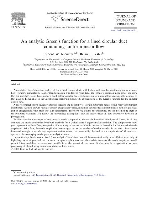
<strong>An</strong> <strong>analytic</strong> Green’s <strong>function</strong> is derived <strong>for</strong> a <strong>lined</strong> <strong>circular</strong> <strong>duct</strong>, both hollow and annular, <strong>containing</strong> uni<strong>for</strong>m mean<br />
flow, from first principles by Fourier trans<strong>for</strong>mation. The derived result takes the <strong>for</strong>m of a common mode series. We show<br />
that the <strong>analytic</strong> Green’s <strong>function</strong> <strong>for</strong> a <strong>lined</strong> hollow <strong>circular</strong> <strong>duct</strong>, <strong>containing</strong> uni<strong>for</strong>m mean flow, is essentially identical to<br />
that used by Tester et al. in the Cargill splice scattering model. The explicit <strong>for</strong>m of the Green’s <strong>function</strong> <strong>for</strong> the annular<br />
<strong>duct</strong> is new.<br />
A more comprehensive causality analysis suggests the possibility of certain upstream modes being really downstream<br />
instabilities. As their growth rates are usually exceptionally large, including these modes as instabilities is both not practical<br />
and in disagreement with most (not all) experiments. There<strong>for</strong>e, we outline the possibility but do not include them in<br />
the presented examples. We follow the ‘‘modelling assumption’’ that all modes decay in their respective direction of<br />
propagation.<br />
To illustrate the advantages of our <strong>analytic</strong> result compared to the matrix inversion technique of Alonso et al., we<br />
compute the mode amplitudes from both methods <strong>for</strong> a typical aircraft engine intake condition. The comparisons show<br />
good agreement without flow, irrespective of how many modes are included in the matrix inversion <strong>for</strong> the numerical mode<br />
amplitudes. With flow, the mode amplitudes do not agree but as the number of modes included in the matrix inversion is<br />
increased, enough to include any important surface waves, the numerically obtained modal amplitudes of Alonso et al.<br />
appear to be converging to the present <strong>analytic</strong>al result.<br />
In practical applications our closed <strong>for</strong>m <strong>analytic</strong> Green’s <strong>function</strong> will be computationally more efficient, especially at<br />
high frequencies of practical interest to aero-engine applications, and the <strong>analytic</strong> <strong>for</strong>m <strong>for</strong> the mode amplitudes could<br />
permit future modelling advances not possible from the numerical equivalent. It also may have application to postprocessing<br />
of phased array measurements inside <strong>lined</strong> <strong>duct</strong>s.<br />
r 2008 Elsevier Ltd. All rights reserved.<br />
Corresponding author.<br />
E-mail addresses: S.W.Rienstra@tue.nl (S.W. Rienstra), brian.j.tester@dsl.pipex.com (B.J. Tester).<br />
0022-460X/$ - see front matter r 2008 Elsevier Ltd. All rights reserved.<br />
doi:10.1016/j.jsv.2008.03.048
Nomenclature<br />
a <strong>duct</strong> diameter<br />
Cm, Dm linear combinations of Bessel <strong>function</strong>s<br />
Jm and Y m<br />
ex, er, ey unit vectors in x, r, y-direction<br />
Em<br />
1. Intro<strong>duct</strong>ion<br />
ARTICLE IN PRESS<br />
S.W. Rienstra, B.J. Tester / Journal of Sound and Vibration 317 (2008) 994–1016 995<br />
auxiliary <strong>function</strong>s of k<br />
F m; Hm; Fm; Hm auxiliary <strong>function</strong>s of r and a<br />
Gðx; x0Þ Green’s <strong>function</strong> (in pressure)<br />
Gmðr; xÞ m-th circumferential Fourier component<br />
of Gðx; x0Þ<br />
HðxÞ Heaviside step <strong>function</strong><br />
h hub-tip ratio (dimensionless hub radius)<br />
Jm, Y m Bessel <strong>function</strong>s of the first and second<br />
kinds of order m<br />
m circumferential modal order<br />
M Mach number<br />
n unit outer normal vector at r ¼ 1<br />
p, v, r, c time-harmonic pressure, velocity,<br />
density, sound speed<br />
x, r, y, taxial, radial, azimuthal angle, time coordinate<br />
Z1, Zh impedance of outer, inner wall<br />
a radial modal wave number; (square root<br />
of minus) eigenvalue of Laplace operator<br />
b ð1 M 2 Þ 1=2<br />
d parameter in numerical procedure<br />
k axial wave number<br />
m radial modal order<br />
s reduced axial wave number<br />
o Helmholtz number (dimensionless angular<br />
frequency)<br />
$ o=b<br />
O o kM<br />
In some recent work, Tester et al. [1,2] described the development and validation of an <strong>analytic</strong>al model <strong>for</strong><br />
the scattering of spinning modes by liner splices, originally derived by Cargill [3] and based on the Kirchhoff<br />
approximation. In his original <strong>for</strong>mulation, Cargill used the hard-walled radial eigen<strong>function</strong>s in the Green’s<br />
<strong>function</strong> <strong>for</strong> a <strong>circular</strong> <strong>duct</strong> <strong>containing</strong> uni<strong>for</strong>m flow. In the recent work [1] an <strong>analytic</strong>, closed <strong>for</strong>m Green’s<br />
<strong>function</strong> was used that was deduced from that given by Tester [4] <strong>for</strong> a <strong>lined</strong> 2D <strong>duct</strong> <strong>containing</strong> uni<strong>for</strong>m flow.<br />
This was assumed to be an approximation although it can be shown that it is a special case of the result<br />
derived by Swinbanks [5] <strong>for</strong> a <strong>lined</strong> 2D <strong>duct</strong> <strong>containing</strong> sheared flow.<br />
In his thesis [6], Schulten gave a version of the spatially Fourier-trans<strong>for</strong>med Green’s <strong>function</strong> of a <strong>lined</strong><br />
annular <strong>duct</strong>, with the suggestion to invert this Fourier-trans<strong>for</strong>m expression numerically. No actual examples<br />
were given, however. Closer to our <strong>for</strong>mulation is the work of Zorumski in Ref. [7]. Not all <strong>for</strong>mulas are<br />
worked out explicitly and no details are given about the numerical evaluation and the role of surface waves.<br />
More recently Alonso et al. [8] have proposed an ‘exact’ Green’s <strong>function</strong> based on the numerical inversion of<br />
a matrix, which has been evaluated in the course of the present work.<br />
In the current work we derive an <strong>analytic</strong> Green’s <strong>function</strong> <strong>for</strong> a <strong>lined</strong> <strong>circular</strong> <strong>duct</strong>, both hollow and<br />
annular, <strong>containing</strong> uni<strong>for</strong>m mean flow, from first principles in closed <strong>for</strong>m, and show that the hollow version<br />
is essentially identical to that used in Ref. [1].<br />
Comparisons are presented with the ‘numerical’ Green’s <strong>function</strong> of Alonso et al. [8,9]. In these presented<br />
examples we assumed that all modes decay in their respective direction of propagation, although more<br />
comprehensive causality analyses [4,10,11], supports the conjecture that some supposedly upstream-running<br />
modes are downstream-running convective instabilities (with the same harmonic time dependence as the<br />
exciting source). Moreover, recently Brambley et al. [12] showed that the liner-mean-flow system may be<br />
absolutely unstable, in which case any convective instability would be meaningless.<br />
The conjectured unstable behaviour is, at least in the realm of the model, confirmed by numerical<br />
calculations in time-domain by Chevaugeon et al. [13]. The physical existence on the other hand is not so clear,<br />
but instabilities have been reported by Ronneberger et al. [14] and Aure´gan et al. [15] in experiments with<br />
impedances of small resistance with predicted (convective) instabilities of small growth rate [10]. For most<br />
impedances met in practice, however (including the ones considered here) the predicted growth rates are<br />
exceptionally large, in which case their physical relevance is questionable as these instabilities have never been<br />
reported [16], and at the same time their inclusion is not practical. For this reason their role is not further
996<br />
explored in the present study, but we will show that, if desired, any such modes may be easily included as a<br />
convective instability in the present <strong>for</strong>mat.<br />
If the liner-mean-flow system is indeed absolutely unstable, including these modes is futile, and we have to<br />
search <strong>for</strong> other, stable models. At present, this is beyond the scope of our paper.<br />
2. The problem<br />
Consider a cylindrical <strong>duct</strong> of radius a40 (possibly annular with inner radius ah), a mean flow of subsonic<br />
Mach number M, sound speed c0 and density r 0 and harmonic pressure and velocity perturbations ~p of<br />
angular frequency ~o (see the sketch Fig. 1). We make dimensionless<br />
~x ¼ xa; ~t ¼ ta=c0; ~o ¼ oc0=a; ~p ¼ r 0c 2 0 Reðpeiot Þ. (1)<br />
The Green <strong>function</strong> Gðx; x0Þ is represented by the pressure field pðxÞ that is excited by a point source at x0, and<br />
satisfies the equation<br />
Note that we use the<br />
r 2 G io þ M q<br />
qx<br />
2<br />
G ¼ dðx x0Þ. (2)<br />
e iot -convention. (3)<br />
The Ingard–Myers impedance boundary condition [17,18] with flow, a linear relation between pressure and<br />
velocity, becomes in terms of the pressure at r ¼ 1<br />
io þ M q<br />
qx<br />
2<br />
qG<br />
G þ ioZ1 ¼ 0 at r ¼ 1. (4)<br />
qr<br />
For a hollow <strong>duct</strong> finiteness of G is assumed at r ¼ 0. For an annular <strong>duct</strong> we have at the inner wall r ¼ h<br />
io þ M q<br />
qx<br />
ARTICLE IN PRESS<br />
S.W. Rienstra, B.J. Tester / Journal of Sound and Vibration 317 (2008) 994–1016<br />
2<br />
qG<br />
G ioZh ¼ 0 at r ¼ h. (5)<br />
qr<br />
Finally, we adopt radiation conditions that says that we only accept solutions that radiate away from the<br />
source position x0.<br />
Fig. 1. Sketch of geometry: <strong>circular</strong> or annular <strong>lined</strong> <strong>duct</strong> with flow.
3. Solution<br />
3.1. The hollow <strong>duct</strong><br />
We represent the delta-<strong>function</strong> by a generalised Fourier series in W and Fourier integral in x<br />
Z 1<br />
dðr r0Þ 1<br />
dðx x0Þ ¼ e<br />
r0 2p 1<br />
ikðx x0Þ 1 X<br />
dk<br />
2p<br />
1<br />
m¼ 1<br />
where 0or0o1, and write accordingly<br />
Gðx; r; W; x0; r0; W0Þ ¼ X1<br />
e<br />
m¼ 1<br />
imðW W0Þ<br />
Gmðr; xÞ ¼ X1<br />
m¼ 1<br />
Substitution of Eqs. (6) and (7) in Eq. (2) yields <strong>for</strong> ^ Gm<br />
with<br />
This has solution<br />
q 2 Gm<br />
^ 1 q<br />
þ<br />
qr2 r<br />
^ Gm<br />
qr<br />
a 2 ¼ O 2<br />
þ a2 m2<br />
r 2<br />
e<br />
^Gm ¼<br />
Z 1<br />
imðW W0Þ<br />
1<br />
e imðW W0Þ . (6)<br />
^Gmðr; kÞe ikðx x0Þ dk. (7)<br />
dðr r0Þ<br />
4p2 , (8)<br />
r0<br />
k 2 ; O ¼ o kM. (9)<br />
^Gmðr; kÞ ¼AðkÞJmðarÞþ 1<br />
8p Hðr r0ÞðJmðar0ÞY mðarÞ Y mðar0ÞJmðarÞÞ, (10)<br />
where Jm and Y m denote the m-th order ordinary Bessel <strong>function</strong>s [19] of the first and second kind, Hðr<br />
denotes the Heaviside step<strong>function</strong>. Use is made of the Wronskian<br />
r0Þ<br />
JmðxÞY 0 mðxÞ Y mðxÞJ 0 2<br />
mðxÞ ¼ .<br />
px<br />
(11)<br />
A prime denotes a derivative to the argument, x. AðkÞ is to be determined from the boundary conditions at<br />
r ¼ 1, which is (assuming uni<strong>for</strong>m convergence) per mode<br />
iO 2 Gm<br />
^ þ oZ1 ^ G 0<br />
m ¼ 0<br />
A prime denotes a derivative to r. This yields<br />
at r ¼ 1. (12)<br />
and thus<br />
where<br />
" #<br />
, (13)<br />
A ¼ 1<br />
8p Y mðar0Þ<br />
ARTICLE IN PRESS<br />
S.W. Rienstra, B.J. Tester / Journal of Sound and Vibration 317 (2008) 994–1016 997<br />
iO 2 Y mðaÞþoaZ1Y 0 mðaÞ iO 2 JmðaÞþoaZ1J 0 Jmðar0Þ<br />
mðaÞ ^Gmðr; kÞ ¼JmðaroÞ iO2F mðr4; aÞþoZ1Hmðr4; aÞ<br />
, (14)<br />
8pEmðkÞ<br />
EmðkÞ ¼iO 2 JmðaÞþoaZ1J 0 mðaÞ, (15a)<br />
F mðr; aÞ ¼JmðaÞY mðarÞ Y mðaÞJmðarÞ, (15b)<br />
Hmðr; aÞ ¼aJ 0 m ðaÞY mðarÞ aY 0 m ðaÞJmðarÞ, (15c)<br />
r4 ¼ maxðr; r0Þ, (15d)<br />
ro ¼ minðr; r0Þ. (15e)
998<br />
By substituting the defining series we find that F m and Hm are <strong>analytic</strong> <strong>function</strong>s of a2 , while both Em and<br />
JmðaroÞ can be written as am times an <strong>analytic</strong> <strong>function</strong> of a2 . As a result, ^ Gmðr; kÞ is a meromorphic <strong>function</strong><br />
of k. It has isolated poles k ¼ kmm , given by EmðkmmÞ¼0. The final solution is found by Fourier back-trans<strong>for</strong>mation: close the integration contour around the lower<br />
half plane <strong>for</strong> x4x0 to enclose the right propagating modes, and the upper half plane <strong>for</strong> xox0 to enclose the<br />
left propagating modes. We find<br />
O 4 mm<br />
ðoammZ1Þ 2<br />
" ! #<br />
2iMOmm<br />
, (16)<br />
oZ1<br />
dEm<br />
¼ oZ1JmðammÞ ðkmmþOmmMÞ 1<br />
dk k¼kmm<br />
m2<br />
a2 mm<br />
and introduce the quantity<br />
Qmm ¼ ðkmmþ OmmMÞ 1 m2<br />
a2 mm<br />
O 4 mm<br />
ðoammZ1Þ 2<br />
" ! #<br />
2iMOmm<br />
,<br />
oZ1<br />
(17)<br />
where the þ, signs apply to right, left-running modes. The integral is evaluated as a sum over the residues in<br />
the poles at k ¼ kþ mm <strong>for</strong> x4x0 and at kmm <strong>for</strong> xox0, in short-hand notation given by<br />
Gmðr; xÞ ¼ 1 X1<br />
i<br />
4<br />
m¼1<br />
JmðammroÞ iO2mm F mðr4; ammÞþoZ1Hmðr4; ammÞ<br />
e<br />
oZ1QmmJmðammÞ ikmmðx x0Þ<br />
, (18)<br />
where amm ¼ aðkmmÞ. From eigenvalue equation Emðk mm Þ¼0 and the Wronskian (11) we obtain<br />
iO 2 mmF mðr4; ammÞþoZ1Hmðr4; ammÞ ¼ ðiO 2 mmY mðammÞþoammZ1Y 0 mðammÞÞJmðammr4Þ ¼<br />
2oZ1<br />
pJmðammÞ Jmðammr4Þ. (19)<br />
So we can skip the distinction between r4 and ro to achieve the soft wall modal expansion<br />
Gmðr; xÞ ¼<br />
1<br />
2pi<br />
X 1<br />
m¼1<br />
JmðammrÞJmðammr0Þ<br />
Q mmJmðammÞ 2 e ikmmðx x0Þ ¼ X 1<br />
m¼1<br />
GmmðrÞe ikmmðx x0Þ . (20)<br />
where <strong>for</strong> x4x0 the sum pertains to the right-running waves, corresponding to the modal wave<br />
numbers k þ mm found in the lower complex half plane, and <strong>for</strong> xox0 the left-running waves, corresponding<br />
to k mm found in the upper complex half plane. Eq. (20) is essentially equivalent to Eq. (2) of Ref. [1]<br />
(see Appendix A).<br />
Only if a mode from the upper half plane is to be interpreted as a right-running instability (see<br />
Refs. [4,10,20]), its contribution is to be excluded from the set of modes <strong>for</strong> xox0 and included in the modes<br />
<strong>for</strong> x4x0. What we essentially do is de<strong>for</strong>m the integration contour into the upper half plane, so the <strong>for</strong>m of<br />
the solution remains exactly the same.<br />
It may be noted that the solution is continuous everywhere, except at the source. As may be expected from<br />
the symmetry of the configuration, the clockwise and anti-clockwise rotating circumferential modes are equal,<br />
i.e. Gmðr; xÞ ¼G mðr; xÞ.<br />
3.2. The annular <strong>duct</strong><br />
ARTICLE IN PRESS<br />
S.W. Rienstra, B.J. Tester / Journal of Sound and Vibration 317 (2008) 994–1016<br />
By choosing suitable variables we can make the solution <strong>for</strong> the annular <strong>duct</strong> similar to the one <strong>for</strong> the<br />
hollow <strong>duct</strong>. First we introduce two independent solutions of the scaled Bessel equation, i.e. the homogeneous<br />
version of Eq. (8), by<br />
Cmðr; aÞ ¼aJmðarÞþbY mðarÞ, (21a)<br />
Dmðr; aÞ ¼cJmðarÞþdY mðarÞ, (21b)
where adabc and Cm is supposed to satisfy the inner wall boundary condition, so a and b satisfy<br />
b<br />
a ¼ iO2JmðahÞ aoZhJ 0 mðahÞ . (22)<br />
ðahÞ<br />
iO 2 Y mðahÞ aoZhY 0 m<br />
Although not necessary <strong>for</strong> the final result, we will assume <strong>for</strong> convenience that ad bc ¼ 1 and<br />
Cm and Dm have now the Wronskian<br />
a ¼ iO 2 Y mðahÞ aoZhY 0 m ðahÞ; b ¼ ðiO2 JmðahÞ aoZhJ 0 m ðahÞÞ.<br />
CmD 0 m DmC 0 m ¼ðad<br />
2 2<br />
bcÞ ¼ .<br />
pr pr<br />
(23)<br />
The prime denotes a derivative to r. The solution of (8) that satisfies the inner wall boundary condition is<br />
^Gmðr; kÞ ¼AðkÞCmðarÞþ 1<br />
8p Hðr r0ÞðCmðr0; aÞDmðr; aÞ Dmðr0; aÞCmðr; aÞÞ. (24)<br />
The boundary condition at r ¼ 1 requires that A equals<br />
A ¼ 1<br />
8p Dmðr0; aÞ<br />
iO 2 Dmð1; aÞþoZ1D 0 "<br />
mð1; aÞ<br />
#<br />
, (25)<br />
and thus<br />
where<br />
iO 2 Cmð1; aÞþoZ1C 0 m ð1; aÞ Cmðr0; aÞ<br />
^Gmðr; kÞ ¼Cmðro; aÞ iO2Fmðr4; aÞþoZ1Hmðr4; aÞ<br />
, (26)<br />
8pEmðkÞ<br />
EmðkÞ ¼iO 2 Cmð1; aÞþoZ1C 0 mð1; aÞ, (27a)<br />
Fmðr; aÞ ¼Cmð1; aÞDmðr; aÞ Dmð1; aÞCmðr; aÞ, (27b)<br />
Hmðr; aÞ ¼C 0 m ð1; aÞDmðr; aÞ D 0 m ð1; aÞCmðr; aÞ. (27c)<br />
Note that Eq. (26) is the equivalent of Eq. (2.71), with Eqs. (2.43), (2.70) and (2.72), of Schulten [6]. Schulten<br />
suggested a numerical approach to evaluate the inverse Fourier trans<strong>for</strong>m, but did not give further details or<br />
examples.<br />
In a similar way as with the hollow <strong>duct</strong> we can show that ^ Gm is a meromorphic <strong>function</strong> in k. Its Fourier<br />
integral that defines Gm can be evaluated in the <strong>for</strong>m of a summation over the residues in kmm, the zeros of<br />
EmðkÞ. From the defining relation EmðkmmÞ ¼0 and the Wronskian we have at k ¼ kmm<br />
iO 2 Fmðr4; ammÞþoZ1Hmðr4; ammÞ ¼ ðiO 2 Dmð1; ammÞþoZ1D 0 mð1; ammÞÞCmðr4; ammÞ<br />
2oZ1<br />
¼<br />
pCmð1; ammÞ Cmðr4; ammÞ,<br />
and so we have the following result, which may be compared with equation (38), of Zorumski [7],<br />
Gmðr; xÞ ¼<br />
¼<br />
Z 1<br />
1<br />
^Gmðr; kÞe ikðx x0Þ dk<br />
1<br />
X1<br />
signðx x0Þ<br />
2pi<br />
ARTICLE IN PRESS<br />
S.W. Rienstra, B.J. Tester / Journal of Sound and Vibration 317 (2008) 994–1016 999<br />
oZ1<br />
E<br />
m¼1<br />
0 Cmðr; ammÞCmðr0; ammÞ<br />
e<br />
ðkmmÞ Cmð1; ammÞ<br />
ikmmðx x0Þ<br />
.
1000<br />
By carefully substituting definitions and Wronskians we obtain<br />
dEm<br />
dk<br />
¼ oZ1 ðkmm þ OmmMÞ<br />
k¼kmm<br />
1 m2<br />
a2 mm<br />
O 4 mm<br />
ðammoZ1Þ 2<br />
" ! #<br />
2iOmmM<br />
Cmð1; ammÞ<br />
oZ1<br />
Furthermore, we have<br />
b da<br />
dk<br />
2oZ1<br />
pCmð1; ammÞ<br />
db<br />
a ¼<br />
dk k¼kmm<br />
2o2Z2 h<br />
p<br />
b da<br />
dk<br />
db<br />
a .<br />
dk k¼kmm<br />
m<br />
ðkmm þ OmmMÞ 1<br />
2<br />
a2 mmh2 O 4 mm<br />
ðammoZhÞ 2<br />
!<br />
þ 2iOmmM<br />
" #<br />
, (28)<br />
hoZh<br />
and Cmðh; aÞ ¼ 2oZh=ph. If we introduce<br />
Q ð1Þ<br />
mm ¼ ðkmm þ OmmMÞ 1 m2<br />
a2 mm<br />
O 4 mm<br />
ðammoZ1Þ 2<br />
" ! #<br />
2iOmmM<br />
,<br />
oZ1<br />
(29a)<br />
Q ðhÞ<br />
mm ¼ ðkmm<br />
m<br />
þ OmmMÞ 1<br />
2<br />
a2 mmh2 O 4 mm<br />
ðammoZhÞ 2<br />
!<br />
þ 2iOmmM<br />
" #<br />
hoZh<br />
(again, the signs apply to right, left-running modes) we have finally in short-hand notation<br />
Gmðr; xÞ ¼<br />
¼ X1<br />
m¼1<br />
1<br />
2pi<br />
X 1<br />
m¼1<br />
Cmðr; ammÞCmðr0; ammÞ<br />
Q ð1Þ<br />
mm Cmð1; ammÞ 2<br />
3.3. Lorentz-type or Prandtl– Glauert trans<strong>for</strong>mation<br />
h 2 Q ðhÞ<br />
mm Cmðh; ammÞ 2 e ikmmðx x0Þ<br />
(29b)<br />
GmmðrÞe ikmmðx x0Þ . (30)<br />
We obtain <strong>for</strong> hard walls some simplification by the following Lorentz-type or Prandtl–Glauert<br />
trans<strong>for</strong>mation. In this case the left and right-running values of amm are symmetric, i.e. aþ mm ¼ amm , while<br />
the corresponding values of kmm are point symmetric in oM=ð1 M2Þ. When we trans<strong>for</strong>m<br />
ffiffiffiffiffiffiffiffiffiffiffiffiffiffiffi<br />
b ¼ 1 M2 p<br />
; x ¼ bX; o ¼ b$; kmm ¼ smm<br />
b<br />
$M<br />
,<br />
Omm ¼ Msmm þ $<br />
;<br />
b<br />
kmm þ OmmM ¼ bsmm,<br />
where we can just write amm and smm without left/right distinction, we obtain<br />
So altogether we have <strong>for</strong> the hollow <strong>duct</strong><br />
Gmðr; xÞ ¼ eiM$ðX X 0Þ X<br />
2pib<br />
1<br />
ARTICLE IN PRESS<br />
S.W. Rienstra, B.J. Tester / Journal of Sound and Vibration 317 (2008) 994–1016<br />
Qmm ¼ bsmm 1 m2<br />
a2 !<br />
mm<br />
.<br />
m¼1<br />
JmðammrÞJmðammr0Þ<br />
!<br />
smm 1 m2<br />
a 2 mm<br />
J2 mðammÞ e ismmjX X 0j<br />
. (31)
Similarly <strong>for</strong> the annular <strong>duct</strong> we get<br />
Gmðr; xÞ ¼ eiM$ðX X 0Þ X<br />
2pib<br />
1<br />
m¼1<br />
Cmðr; ammÞCmðr0; ammÞe ismmjX X 0j<br />
" !<br />
! #. (32)<br />
smm 1 m2<br />
a 2 mm<br />
C 2 m ð1; ammÞ h 2 1<br />
m 2<br />
a 2 mm h2<br />
C 2 mðh; ammÞ<br />
Note that apart from the term exp½iM$ðX X 0ÞŠ, Gm only depends on M 2 and jx x0j. There<strong>for</strong>e, jGmðx; rÞj<br />
is symmetric in x x0 <strong>for</strong> any subsonic Mach number.<br />
4. Unstable modes as artifacts of the modelling?<br />
The question of including possible instabilities is not resolved yet. Let us try to summarise our position:<br />
(i) Sound occurs mostly in the <strong>for</strong>m of very small perturbations, and it seems well justified to model it by<br />
some <strong>for</strong>m of linearised Euler equations.<br />
(ii) Viscous boundary layers of high-Reynolds flows along walls are, in the aero-engine applications we have<br />
in mind, much thinner than a characteristic wave length.<br />
(iii) Points (i) and (ii) together led Ingard [17] and later Myers [18] to derive their impedance wall condition <strong>for</strong><br />
sound at an impedance wall in a mean flow with slip at the wall (i.e. the boundary layer is collapsed into a<br />
vortex sheet [21]). The aero-acoustics community followed them and now the Ingard–Myers boundary<br />
condition is the state-of-the-art <strong>for</strong> this kind of mean flows.<br />
(iv) However, more refined analyses (see Appendix B) as well as numerical time-domain results [13] indicate<br />
that the wall vortex sheet along the <strong>lined</strong> wall may be convectively, or even absolutely [12] unstable. If we<br />
blindly followed the model, this would imply that we had to include these instabilities. Maybe this is right<br />
<strong>for</strong> impedances of small resistance with instabilities of small growth rates. For the majority of cases,<br />
however, the predicted unstable mode has a large growth rate [10], and we believe that in these cases the<br />
instabilities are just artifacts of the model. In physical reality no such instabilities are found [16]. The<br />
reason is not clear yet: maybe any instability of the wall vortex sheet is immediately blocked by the wall;<br />
maybe the actual wall boundary layer is too thick, cf. Refs. [22,23]; or perhaps our liner-mean-flow model<br />
is too simple [12]. In other words: point (ii) is incompatible with point (i).<br />
(v) So we have here three options: (1) include the instability, knowing that the found field is the solution of a<br />
questionable model; (2) increase the complexity of the model and thus destroying any possibility of<br />
<strong>analytic</strong>al solutions; and (3) ignore, as a ‘‘modelling assumption’’, any instability.<br />
For the examples to be given below, where the growth rates of the candidate instability are very large, we<br />
chose option (3).<br />
5. Numerical examples<br />
ARTICLE IN PRESS<br />
S.W. Rienstra, B.J. Tester / Journal of Sound and Vibration 317 (2008) 994–1016 1001<br />
Numerical evaluation of the pressure field is not too difficult if we are able to find all the modal<br />
wavenumbers kmm necessary <strong>for</strong> the required accuracy. We adopted the method, out<strong>lined</strong> in Ref. [10], which is<br />
based on continuation from the (assumed easily found) hard-wall values to the sought soft-wall values. The<br />
crux of the method is that we start from a suitable hard-wall direction jZj !1in the complex impedance<br />
plane in order to capture all wavenumbers occurring at the finite impedance, say, Z0. This is not entirely<br />
straight<strong>for</strong>ward. When we trace the wavenumbers backwards, from the soft-wall to the hard-wall values, there<br />
are certain intervals of argðZÞ where some wavenumbers disappear to infinity. These would be impossible to<br />
find if we started there with our <strong>for</strong>ward search. It transpires that a search along vertical lines in the complex Z<br />
plane, from Z ¼ ReðZ0Þ i1 when M ¼ 0 and from Z ¼ ReðZ0Þþi signðMÞ1 otherwise, guarantees finding<br />
of all the wave numbers.
1002<br />
To be completely specific, we define Z0 ¼ R0 þ iX 0 and parameterise<br />
1<br />
YðlÞ ¼ ZðlÞ ¼R0 þ id cotðlÞ; 0plpl0 ¼ arccotðdX 0Þ, (33)<br />
where d ¼ signðMÞ if Ma0 andd¼ any l by the identity<br />
1ifM ¼ 0. Solutions k <strong>for</strong> the hollow <strong>duct</strong> are now implicitly given <strong>for</strong><br />
f ðk; YÞ ¼YEmðkÞ ¼iO 2 YJmðaÞþoaJ 0 mðaÞ 0. (34)<br />
We know the hard-wall solutions corresponding to l ¼ 0. After differentiation of f to l we obtain an ordinary<br />
differential equation in k that can be integrated numerically as an initial value problem. We thus pick a mode<br />
by choosing an initial value and solve numerically by standard methods<br />
G m<br />
ARTICLE IN PRESS<br />
S.W. Rienstra, B.J. Tester / Journal of Sound and Vibration 317 (2008) 994–1016<br />
100<br />
80<br />
60<br />
40<br />
20<br />
0<br />
−20<br />
−40<br />
−60<br />
−80<br />
df qf<br />
¼<br />
dl qk<br />
dk<br />
dl<br />
qf dY<br />
þ ¼ 0 (35)<br />
qY dl<br />
−100<br />
−20 0 20 40 60 80<br />
0.2<br />
0.1<br />
0<br />
−0.1<br />
−0.2<br />
−1 −0.5 0<br />
x<br />
0.5 1<br />
Fig. 2. 400 Modes at r ¼ r0 ¼ 0:7 with M ¼ 0:5, o ¼ 10, h ¼ 0:3, m ¼ 3, Z1 ¼ 1 i, Zh ¼ 1 þ i: (a) complex kmm-plane; and<br />
(b) ReðGmÞ (– –), ImðGmÞ ( ), jGmj (—).
ARTICLE IN PRESS<br />
S.W. Rienstra, B.J. Tester / Journal of Sound and Vibration 317 (2008) 994–1016 1003<br />
to obtain an approximation <strong>for</strong> kðl0Þ. If we deal with a surface wave, we divide f by Jm. The accuracy of the<br />
final result may be optimised by one or two Newton iterations. For an annular <strong>duct</strong> we do something similar<br />
with f ¼ Y 1Y hEm.<br />
The number of terms we need <strong>for</strong> Gmðr; xÞ is dependent on the convergence rate, which depends greatly on<br />
the value of x x0. Whenever x x0a0 the convergence is exponentially fast, and hence absolute, through<br />
the factor expð ikmmðx x0ÞÞ. Only when x ¼ x0 the series converges conditionally when rar0, and when<br />
r ¼ r0 it diverges (deceivingly) slowly like a harmonic series ð P m 1 lnðm maxÞÞ.<br />
As the series at the left and right side of the source plane are not symmetric whenever Ma0, we will have a<br />
discontinuity at x ¼ x0 <strong>for</strong> any finite number of terms. This jump is a marked evidence of any insufficient<br />
accuracy and will disappear when enough terms are included. However, it should be noted that also when M<br />
40<br />
30<br />
20<br />
10<br />
0<br />
−10<br />
−20<br />
−30<br />
−40<br />
−40 −30 −20 −10 0 10 20 30 40<br />
400<br />
300<br />
200<br />
100<br />
0<br />
−100<br />
−200<br />
−300<br />
−400<br />
−140 −120 −100 −80 −60 −40 −20 0 20 40 60<br />
Fig. 3. Location of kmm <strong>for</strong> comparable cases without flow (a) and with flow (b). In both cases is Z ¼ 2:5 and m ¼ 0, while o ¼ 31:354 with<br />
M ¼ 0 (a) and o ¼ 28 with M ¼ 0:45 (b). Note with flow the very well cut-off surface wave, which nevertheless plays a role near the wall<br />
around the source plane.
1004<br />
ARTICLE IN PRESS<br />
tends to zero the jump will disappear, but only because the solution becomes symmetric. It has no relation to<br />
the accuracy of the series.<br />
To illustrate the points noted above, we present the m ¼ 3—circumferential component Gm in Fig. 2 <strong>for</strong> a<br />
source at x0 ¼ 0, r0 ¼ 0:7 and o ¼ 10 in an annular <strong>duct</strong> with h ¼ 0:3, Z1 ¼ 1 i and Zh ¼ 1 þ i and a mean<br />
flow of M ¼ 0:5. Gm is plotted at r ¼ 0:7 <strong>for</strong> 1pxp1. In addition the complex axial wave numbers kmm are<br />
presented. We observe two surface waves in the first quadrant (technically, these are both candidate <strong>for</strong><br />
instability, but, as indicated above, this fact has no bearing on the present solution). In order to make sure that<br />
−<br />
|Gmµ| Phase (G− mµ )<br />
S.W. Rienstra, B.J. Tester / Journal of Sound and Vibration 317 (2008) 994–1016<br />
10 0<br />
10 −1<br />
10 −2<br />
10 0 10 1<br />
10 −3<br />
Radial Mode Number<br />
3<br />
2<br />
1<br />
0<br />
−1<br />
−2<br />
−3<br />
10 0 10 1<br />
Radial Mode Number<br />
Fig. 4. Green’s <strong>function</strong> mode amplitude: modulus (a) and phase (b) (o ¼ 31:354, M ¼ 0, Z1 ¼ 2:5, r0 ¼ 1, cut-off ratio ¼ 0:28).<br />
Numerical and <strong>analytic</strong> results indistinguishable. Left and right running modes the same.<br />
28<br />
24<br />
20<br />
16<br />
12<br />
8<br />
4<br />
0
ARTICLE IN PRESS<br />
the series has converged in any plotted value of xax0, that is <strong>for</strong> 400pjx x0jb1, say, we used 400 radial<br />
modes, but the difference with less than that is only visible very near the source.<br />
In addition to this example <strong>for</strong> annular <strong>duct</strong>s we have compared our <strong>analytic</strong> Green’s <strong>function</strong> <strong>for</strong> hollow<br />
<strong>duct</strong>s with the ‘numerical’ Green’s <strong>function</strong> described by Alonso et al. [8]. We consider two cases, one with no<br />
mean flow, M ¼ 0, and one with a typical ‘intake’ Mach number of M ¼ 0:45. A typical non-dimensional<br />
frequency is o ¼ 28 <strong>for</strong> the flow case and we choose o ¼ 31:354 <strong>for</strong> the zero flow case so that the cut-off ratio<br />
of the highest hardwall cut-on mode is about the same <strong>for</strong> both cases. The impedance is Z1 ¼ 2:5 i0 in both<br />
cases. The number of cut-off modes included in the evaluation of the <strong>analytic</strong>al and numerical Green’s<br />
<strong>function</strong> evaluation corresponds to a cut-off ratio of 0.28 (i.e. the number of modes is set equal to the number<br />
of modes above that cut-off ratio that would exist if the <strong>duct</strong> was hard-walled) and only the positive modes in<br />
SPL at r=1<br />
40<br />
20<br />
0<br />
−20<br />
−40<br />
−0.04 −0.02 0<br />
x−x0 0.02 0.04<br />
Phase at r=1<br />
3<br />
2<br />
1<br />
0<br />
−1<br />
−2<br />
−3<br />
28<br />
24<br />
20<br />
16<br />
12<br />
8<br />
4<br />
0<br />
Total<br />
−0.04 −0.02 0<br />
x−x0 0.02 0.04<br />
Fig. 5. Axial variation of Green’s <strong>function</strong> amplitudes per azimuthal mode, SPL ¼ 20 logðjGmjÞ, and total field SPL (o ¼ 31:354, M ¼ 0,<br />
Z1 ¼ 2:5, r0 ¼ 1, cut-off ratio ¼ 0:28). Numerical and <strong>analytic</strong> results indistinguishable. Mode amplitude (a) and phase (b) on each side of<br />
source plane.<br />
±<br />
|Gm |, dB<br />
0<br />
−10<br />
S.W. Rienstra, B.J. Tester / Journal of Sound and Vibration 317 (2008) 994–1016 1005<br />
−20<br />
−30<br />
−40<br />
28<br />
24<br />
20<br />
16<br />
12<br />
8<br />
4<br />
0<br />
0 50 100<br />
Radial Mode Number<br />
150 200<br />
Phase (G± m ), radians<br />
3<br />
2<br />
1<br />
0<br />
−1<br />
−2<br />
−3<br />
0 50 100<br />
Radial Mode Number<br />
150 200<br />
Fig. 6. <strong>An</strong>alytic Green’s <strong>function</strong> azimuthal mode amplitude variation with increasing radial mode number count m max; there is no finite<br />
asymptotic limit at the source position, as each azimuthal mode amplitude varies like logðm maxÞ (o ¼ 31:354, M ¼ 0, Z1 ¼ 2:5, r0 ¼ 1, <strong>for</strong><br />
min. cut-off ratio of 0.07). Left and right running modes: modulus (a) and phase (b).
1006<br />
ARTICLE IN PRESS<br />
the cut-on range 28 ð 4Þ 0 are shown. The source position is always at the wall, r0 ¼ 1, and the observer<br />
position is also on the wall, r ¼ 1, and at the same azimuthal location as the source but at a variable axial<br />
distance from the source both to the left and right of the source plane.<br />
We should explain that this unusual combination of source/observer positions is not particularly relevant to<br />
the computation of liner per<strong>for</strong>mance—where x x0 would be typically the liner length <strong>for</strong> example—but it is<br />
relevant to the modelling of liner splice effects and other sources of scattering. Then the liner splice is the<br />
‘‘source’’ of the scattered field and one requires that field in modal <strong>for</strong>m in the direct vicinity of that source.<br />
The typical location of the axial wave numbers in the complex k-plane <strong>for</strong> both cases is presented in Figs. 3.<br />
The presence of a very well cut-off surface wave in the case with flow anticipates the convergence problems to<br />
be reported below when the source is positioned at the wall, right inside the region where the surface wave is<br />
important.<br />
For the first (zero flow) case, we show in Fig. 4 the absolute value (or modulus) and corresponding phase of<br />
each radial mode amplitude as a <strong>function</strong> of radial mode number. Each mode is plotted only once, as in this<br />
zero-flow case the left and right running modes are the same, while the numerical [8] and <strong>analytic</strong>al results<br />
agree to better than 10 14 . The same is true <strong>for</strong> the total field, as illustrated in Fig. 5. Here we have summed the<br />
radial modes <strong>for</strong> each azimuthal mode in the Green’s <strong>function</strong> and plotted the axial variation of each<br />
|G − mµ |<br />
|G − mµ |<br />
10 0<br />
10 −1<br />
10 −2<br />
10 0 10 1<br />
10 −3<br />
Radial Mode Number<br />
10 0<br />
10 −1<br />
10 −2<br />
10 −3<br />
S.W. Rienstra, B.J. Tester / Journal of Sound and Vibration 317 (2008) 994–1016<br />
10 0 10 1<br />
Radial Mode Number<br />
28<br />
24<br />
20<br />
16<br />
12<br />
8<br />
4<br />
0<br />
|G + mµ |<br />
|G+ mµ |<br />
10 0<br />
10 −1<br />
10 −2<br />
10 −3<br />
10 0<br />
10 −1<br />
10 −2<br />
10 0 10 1<br />
Radial Mode Number<br />
10 0 10 1<br />
10 −3<br />
Radial Mode Number<br />
Fig. 7. <strong>An</strong>alytic v. numerical Green’s <strong>function</strong> mode amplitude: modulus (o ¼ 28, M ¼ 0:45, Z1 ¼ 2:5, r0 ¼ 1, cut-off ratio ¼ 0:28).<br />
<strong>An</strong>alytical: left (a) and right (b) running modes. Numerical: left (c) and right (d) running modes.
ARTICLE IN PRESS<br />
azimuthal mode (modulus and phase) <strong>for</strong> a short distance to the left and right of the source plane, as well as<br />
the total Green’s <strong>function</strong>. Although these fields are continuous at the source, this does not mean that we have<br />
a converged value at the source plane (maybe near the source). On the contrary, it can be seen (Fig. 6, left) that<br />
none of the azimuthal mode amplitudes converge to a finite limit, indeed because the field diverges at the<br />
source position r ¼ r0. We cannot demonstrate this as easily with the numerical Green’s <strong>function</strong>, as we have<br />
to invert, <strong>for</strong> each azimuthal mode number, a 2N 2N matrix where N is the number of radial modes. As we<br />
increase N much above 70, depending on the azimuthal mode number, the matrix appears to become ill<br />
conditioned and we can no longer solve <strong>for</strong> the numerical mode amplitudes. However, below that limit the rate<br />
of convergence appears to be similar to that of the <strong>analytic</strong>al Green’s <strong>function</strong>.<br />
For the flow case, the picture changes in some ways. In particular, we lose the left/right symmetry <strong>for</strong> the<br />
mode amplitudes, as is seen in Fig. 7. InFig. 8 we show the ratio of the <strong>analytic</strong>al and numerical mode<br />
amplitudes and it can be seen that the two results agree to better than 20% in modulus <strong>for</strong> the cut-on modes<br />
although these differences appear to grow without limit <strong>for</strong> the very well cut-off modes. As a result the axial<br />
variation of the <strong>analytic</strong>al and numerical Green’s <strong>function</strong> agree fairly well away from the source plane, but at<br />
and near the source plane there are significant differences, <strong>for</strong>eshadowing the not yet included surface wave<br />
(see below). In particular, Fig. 9 shows that, with this number of modes, the <strong>analytic</strong>al and numerical Green’s<br />
<strong>function</strong> have a large but different discontinuity at the source plane.<br />
|G −<br />
| Ratio<br />
mµ<br />
Phase Diff (G −<br />
), Radians<br />
mµ<br />
3<br />
2.5<br />
2<br />
1.5<br />
1<br />
0.5<br />
0.5<br />
0<br />
0 10 20 30 40 50 60<br />
1<br />
0<br />
−0.5<br />
S.W. Rienstra, B.J. Tester / Journal of Sound and Vibration 317 (2008) 994–1016 1007<br />
Radial Mode Number<br />
−1<br />
0 10 20 30 40 50 60<br />
Radial Mode Number<br />
|G +<br />
| Ratio<br />
mµ<br />
Phase Diff (G −+<br />
), Radians<br />
mµ<br />
3<br />
2.5<br />
2<br />
1.5<br />
1<br />
0.5<br />
−0.5<br />
0<br />
0 10 20 30 40 50 60<br />
1<br />
0.5<br />
0<br />
28<br />
24<br />
20<br />
16<br />
12<br />
8<br />
4<br />
0<br />
Radial Mode Number<br />
−1<br />
0 10 20 30 40 50 60<br />
Radial Mode Number<br />
Fig. 8. Ratio of numerical over <strong>analytic</strong> Green’s <strong>function</strong> mode amplitudes (o ¼ 28, M ¼ 0:45, Z1 ¼ 2:5, r0 ¼ 1; numerical based on 40<br />
cut-off modes). Modulus: left (a) and right (b) running modes. Phase: left (c) and right (d) running modes.
1008<br />
ARTICLE IN PRESS<br />
However, with reference to the zero-flow case, if we increase the number of cut-off modes to a cut-off<br />
ratio of 0:07, the convergence behaviour is similar in some ways, but strikingly different <strong>for</strong> the modes<br />
to the right of the source plane as shown in Fig. 10. Here there are dramatic jumps in the azimuthal<br />
mode amplitudes in the region of radial mode orders 80–95, which has been identified as the effect of a very<br />
well cut-off ‘surface wave’ which makes a large contribution at and near the <strong>duct</strong> wall (see Fig. 3). Once this<br />
has been included, the convergence is similar to the zero flow case. When this high number of radial<br />
modes is included in the <strong>analytic</strong>al Green’s <strong>function</strong>, the discontinuity at the source plane disappears as shown<br />
in Fig. 11.<br />
The missing surface wave also explains the deviating ratio between <strong>analytic</strong>al and numerical mode<br />
amplitudes in Fig. 8. The numerical Green’s <strong>function</strong> with its en<strong>for</strong>ced continuity at the source plane, when<br />
evaluated with an insufficient number of cut-off modes, attempts to achieve that continuity by slightly<br />
adjusting the amplitude of the cut-on modes and making larger adjustments to the well cut-off modes. When<br />
large enough modes are taken, such that any missing surface waves are included, this error will no doubt<br />
reduce, but the necessary number of modes may be high (as the present example shows).<br />
SPL at r = 1<br />
SPL at r=1<br />
40<br />
20<br />
0<br />
−20<br />
−40<br />
−0.04 −0.02 0<br />
x−x0 0.02 0.04<br />
40<br />
20<br />
0<br />
−20<br />
S.W. Rienstra, B.J. Tester / Journal of Sound and Vibration 317 (2008) 994–1016<br />
−40<br />
−0.04 −0.02 0<br />
x−x0 0.02 0.04<br />
Phase at r=1<br />
Phase at r=1<br />
3<br />
2<br />
1<br />
0<br />
−1<br />
−2<br />
−3<br />
−0.04 −0.02 0<br />
x−x0 0.02 0.04<br />
3<br />
2<br />
1<br />
0<br />
−1<br />
−2<br />
−3<br />
28<br />
24<br />
20<br />
16<br />
12<br />
8<br />
4<br />
0<br />
Total<br />
−0.04 −0.02 0<br />
x−x0 0.02 0.04<br />
Fig. 9. Axial variation of <strong>analytic</strong> and numerical Green’s <strong>function</strong> amplitudes per azimuthal mode, SPL ¼ 20 logðjGmjÞ, and total field<br />
SPL (o ¼ 28, M ¼ 0:45, Z1 ¼ 2:5, r0 ¼ 1, cut-off ratio ¼ 0:28). <strong>An</strong>alytical mode amplitude (a) and phase (b), and numerical mode<br />
amplitude (c) and phase (d) on each side of source plane.
ARTICLE IN PRESS<br />
Finally in order to show the behaviour of the <strong>analytic</strong>al and numerical Green’s <strong>function</strong> continuity at the<br />
source plane away from the source position, Fig. 12 <strong>for</strong> the zero flow case, shows the variation in the radial<br />
direction at the source plane, at the same azimuthal angle as the source, of the modulus of the azimuthal mode<br />
number amplitudes and also the total field, in dB. Shown <strong>for</strong> comparison is the free-field Green’s <strong>function</strong><br />
1=ð4pRÞ, where R is the distance from the source at r0 ¼ 1, multiplied by a plane wave correction to account<br />
<strong>for</strong> the reflection or image source in the <strong>lined</strong> <strong>duct</strong> wall equal to 2Z1=ðZ1 þ 1Þ. It can be seen that the<br />
agreement between the <strong>analytic</strong>al and corrected free-field Green’s <strong>function</strong> <strong>for</strong> this zero flow case is very good<br />
and that continuity (i.e. the total field made up of right running modes ðþÞ equals the total field made up of<br />
left running modes ð Þ) at the source plane is achieved away from the source position—these are<br />
indistinguishable <strong>for</strong> this zero flow case. Here we have decreased the cut-off ratio to 0.07 <strong>for</strong> the <strong>analytic</strong><br />
Green’s <strong>function</strong> evaluation but had to limit the numerical Green’s <strong>function</strong> evaluation to 40 cut-off radial<br />
modes to avoid serious corruption of the solution due to ill-conditioned matrices <strong>for</strong> the higher azimuthal<br />
modes.<br />
The corresponding radial dependence <strong>for</strong> the mean flow case is shown in Fig. 13. Here we have also used a<br />
cut-off ratio of 0.07 <strong>for</strong> the <strong>analytic</strong> Green’s <strong>function</strong> evaluation and again 40 cut-off radial modes <strong>for</strong> the<br />
numerical version. This figure shows that we achieved comparable accuracy to the no-flow case in respect of<br />
continuity at the source plane and the agreement with the free-field Green’s <strong>function</strong> verifies that we have<br />
|G− m |, dB<br />
Phase(G− m ), radians<br />
0<br />
−10<br />
−20<br />
−30<br />
−40<br />
0 50 100<br />
Radial Mode Number<br />
150 200<br />
3<br />
2<br />
1<br />
0<br />
−1<br />
−2<br />
S.W. Rienstra, B.J. Tester / Journal of Sound and Vibration 317 (2008) 994–1016 1009<br />
−3<br />
0 50 100<br />
Radial Mode Number<br />
150 200<br />
|G + m |, dB<br />
Phase(G + m ), radians<br />
0<br />
−10<br />
−20<br />
−30<br />
−40<br />
28<br />
24<br />
20<br />
16<br />
12<br />
8<br />
4<br />
0<br />
0 50 100<br />
Radial Mode Number<br />
150 200<br />
3<br />
2<br />
1<br />
0<br />
−1<br />
−2<br />
−3<br />
0 50 100<br />
Radial Mode Number<br />
150 200<br />
Fig. 10. <strong>An</strong>alytic Green’s <strong>function</strong> azimuthal mode amplitude convergence (o ¼ 28, M ¼ 0:45, Z1 ¼ 2:5, r0 ¼ 1, cut-off ratio ¼ 0:07).<br />
Behaviour of left (a) and right (b) running mode amplitude, left (c) and right (d) running mode phase.
1010<br />
a valid <strong>analytic</strong>al description of the Green’s <strong>function</strong> in the presence of a uni<strong>for</strong>m mean flow. The effects of<br />
mean flow on the free-field Green’s <strong>function</strong> have been neglected here as these are small <strong>for</strong> radiation normal<br />
to the mean flow.<br />
6. Conclusions<br />
ARTICLE IN PRESS<br />
Since the <strong>lined</strong>-wall flow-<strong>duct</strong> modes are not orthogonal, or bi-orthogonal to any convenient set of basis<br />
<strong>function</strong>s, it is not possible to obtain a modal series expansion of the Green’s <strong>function</strong> in the classical way,<br />
e.g. as out<strong>lined</strong> in Ref. [24]. It is possible to set up a linear system <strong>for</strong> a finite number of amplitudes either by<br />
utilising the generalised bi-orthogonality relation of Kraft and Wells [25], or directly as in Alonso and<br />
Burdisso [8,9], but the results are approximations, depending on the number of terms. We have followed<br />
another approach, by representing the solution as a Fourier integral and converting it into a modal series by<br />
summation over the residues. The resulting amplitudes are exact and explicit.<br />
SPL at r=1<br />
SPL at r=1<br />
40<br />
20<br />
0<br />
−20<br />
−40<br />
−0.04 −0.02 0 0.02 0.04<br />
40<br />
20<br />
0<br />
−20<br />
S.W. Rienstra, B.J. Tester / Journal of Sound and Vibration 317 (2008) 994–1016<br />
x−x 0<br />
−40<br />
−0.04 −0.02 0 0.02 0.04<br />
x−x 0<br />
Phase at r=1<br />
Phase at r=1<br />
3<br />
2<br />
1<br />
0<br />
−1<br />
−2<br />
−3<br />
−0.04 −0.02 0 0.02 0.04<br />
3<br />
2<br />
1<br />
0<br />
−1<br />
−2<br />
−3<br />
28<br />
24<br />
20<br />
16<br />
12<br />
8<br />
4<br />
0<br />
Total<br />
x−x 0<br />
−0.04 −0.02 0 0.02 0.04<br />
Fig. 11. Axial variation of <strong>analytic</strong> and numerical Green’s <strong>function</strong> amplitudes per azimuthal mode, SPL ¼ 20 logðjGmjÞ, and total field<br />
SPL (o ¼ 28, M ¼ 0:45, Z1 ¼ 2:5, r0 ¼ 1, <strong>analytic</strong>: cut-off ratio ¼ 0:07, numerical: limited to 40 cut-off modes). <strong>An</strong>alytical mode<br />
amplitude (a) and phase (b), numerical mode amplitude (c) and phase (d) on each side of the source plane.<br />
x−x 0
SPL, dB<br />
50<br />
40<br />
30<br />
20<br />
10<br />
0<br />
−10<br />
−20<br />
−30<br />
−40<br />
−50<br />
0.8 0.85 0.9<br />
Radius (r)<br />
0.95 1<br />
ARTICLE IN PRESS<br />
S.W. Rienstra, B.J. Tester / Journal of Sound and Vibration 317 (2008) 994–1016 1011<br />
28+<br />
28−<br />
24+<br />
24−<br />
20+<br />
20−<br />
16+<br />
16−<br />
12+<br />
12−<br />
8+<br />
8−<br />
4+<br />
4−<br />
0+<br />
0−<br />
Total+<br />
Total−<br />
Free−field<br />
−50<br />
0.8 0.85 0.9<br />
Radius (r)<br />
0.95 1<br />
Fig. 12. Radial variation without flow of <strong>analytic</strong> and numerical Green’s <strong>function</strong> amplitudes per azimuthal mode, SPL ¼ 20 logðjGmjÞ,<br />
and total field SPL v. free-field Green’s <strong>function</strong> þ reflected SPL (o ¼ 31:354, M ¼ 0, Z1 ¼ 2:5, r0 ¼ 1, <strong>analytic</strong>: cut-off ratio ¼ 0:07,<br />
numerical: limited to 40 cut-off modes). <strong>An</strong>alytical (a), numerical (b). NB: The left and right running modal (<strong>analytic</strong> and numerical)<br />
Green’s <strong>function</strong>s, labelled Totalþ, Total , are indistinguishable in these no-flow results and oscillate about the Free-field Green’s<br />
<strong>function</strong>, which decays monotonically away from the source at r ¼ 1.<br />
The issue of a possible instability is still an open question. Causality considerations suggest, at least in the<br />
linear model, the presence of convective or even absolute instabilities. This has found support by numerical<br />
results in time domain [13]. Also experimentally there is evidence [14,15], at least <strong>for</strong> impedances of small<br />
resistance. In most cases, however, the exponentially large fields that would result have little resemblance with<br />
physical reality. There<strong>for</strong>e, we have not included any such instability in the presented numerical results and<br />
adopted stability of the solution as modelling assumption.<br />
Comparison of our <strong>analytic</strong>al mode amplitudes (<strong>for</strong> the hollow <strong>duct</strong> version of our solution) with the<br />
numerical solution of Alonso et al. showed a good agreement without mean flow, irrespective of how<br />
many modes are included in the matrix inversion <strong>for</strong> the numerical mode amplitudes. A large number of<br />
modes are required <strong>for</strong> convergence near the source. With flow, the mode amplitudes do not agree but<br />
as the number of modes included in the matrix inversion is increased, enough to include all important surface<br />
SPL, dB<br />
50<br />
40<br />
30<br />
20<br />
10<br />
0<br />
−10<br />
−20<br />
−30<br />
−40
1012<br />
(a)<br />
SPL, dB<br />
50<br />
40<br />
30<br />
20<br />
10<br />
0<br />
−10<br />
−20<br />
−30<br />
−40<br />
28+<br />
28−<br />
24+<br />
24−<br />
20+<br />
20−<br />
16+<br />
16−<br />
12+<br />
12<br />
8+<br />
8−<br />
4+<br />
4−<br />
0+<br />
0−<br />
Total+<br />
Total−<br />
Free−field<br />
−50<br />
0.8 0.85 0.9<br />
Radius (r)<br />
0.95 1<br />
ARTICLE IN PRESS<br />
S.W. Rienstra, B.J. Tester / Journal of Sound and Vibration 317 (2008) 994–1016<br />
waves, the numerically obtained modal amplitudes of Alonso et al. appear to be converging to the present<br />
<strong>analytic</strong>al result.<br />
Indeed, this numerical exercise showed the importance of including all relevant modes, especially when they<br />
behave as surface waves. When source and observer position are at the wall, they are in the regime of the<br />
surface wave, so irrespective of the modal decay rate, overlooking the surface wave produces an unconverged<br />
solution and a detectable discontinuity of the field at the source. A reliable method to find all modes, based on<br />
their behaviour with impedance Z along lines parallel to the imaginary axis is described in some detail.<br />
In practical applications our closed <strong>for</strong>m <strong>analytic</strong> Green’s <strong>function</strong> will be computationally more efficient,<br />
especially at high frequencies of practical interest to aero-engine applications, and the <strong>analytic</strong> <strong>for</strong>m <strong>for</strong> the<br />
mode amplitudes could permit future modelling advances not possible from the numerical equivalent. For<br />
example it has already been applied to post-processing of phased array measurements inside <strong>lined</strong> <strong>duct</strong>s by<br />
Sijtsma [26].<br />
(b)<br />
SPL, dB<br />
50<br />
40<br />
30<br />
20<br />
10<br />
0<br />
−10<br />
−20<br />
−30<br />
−40<br />
−50<br />
0.8<br />
0.85 0.9<br />
Radius (r)<br />
0.95 1<br />
Fig. 13. Radial variation with flow of <strong>analytic</strong> and numerical Green’s <strong>function</strong> amplitudes per azimuthal mode, SPL ¼ 20 logðjGmjÞ, and<br />
total field SPL v. free-field Green’s <strong>function</strong> + reflected SPL (o ¼ 28, M ¼ 0:45, Z1 ¼ 2:5, r0 ¼ 1, <strong>analytic</strong>: cut-off ratio ¼ 0:07,<br />
numerical: limited to 40 cut-off modes). <strong>An</strong>alytical (a), numerical (b).<br />
NB: The left and right running <strong>analytic</strong> modal Green’s <strong>function</strong>s, labelled Totalþ, Total , can just be distinguished in these with-flow<br />
results and more so <strong>for</strong> the numerical Green’s <strong>function</strong>, both oscillating about the monotonic Free-field Green’s <strong>function</strong>.
Acknowledgements<br />
The contribution of SWR was partly carried out during a visit of the Department of Applied Mathematics<br />
and Theoretical Physics of the University of Cambridge, financed by a grant from the Royal Society, in the<br />
Spring of 2004. We are very grateful to both the Royal Society, the Department and Professor Nigel Peake <strong>for</strong><br />
their support, hospitality, inspiring discussions and interest.<br />
We acknowledge the discussions with Ed Brambley (DAMTP, Cambridge University).<br />
We are grateful to ms dr Heike JJ Gramberg and dr Nick C Ovenden <strong>for</strong> skillfully implementing the routine<br />
(34) to find all modal wave numbers. The present results would not have been possible without it.<br />
Appendix A. Corrected <strong>for</strong>m of Tester et al. [1]<br />
Un<strong>for</strong>tunately, Eq. (2) of Tester et al. [1] contains some minor typographical errors. The corrected <strong>for</strong>m is<br />
given by<br />
Gðx; r; yjx0; r0; y0Þ ¼<br />
1<br />
2pi<br />
X<br />
m;n<br />
JmðkrmnrÞJmðk rmnr0Þ exp½ ikxmnjx x0jŠ exp½ imðy y0ÞŠ,<br />
wmnLmn where kxmn ¼ð Mxk þ wmnÞ=ð1 M2 xÞ, wmn ¼ðk2 ð1 M2 x rmnÞ1=2 with ImðwmnÞp0, and<br />
Lmn ¼ J 0 mðkrmnÞ2 þ JmðkrmnÞ 2 1 m2<br />
" #<br />
2iMxð1 kxmnMx=kÞ .<br />
Zwmn This is equivalent to the present <strong>for</strong>m if we identify o ¼ k, amm ¼ krmn, kmm ¼ kxmn, ðkmm þ OmmMÞ ¼ w mn<br />
and Q mmJmðammÞ 2 ¼ w mnLmn, with the understanding that the upper sign is taken <strong>for</strong> the x4x0 (i.e. the right<br />
running modes) and the lower sign <strong>for</strong> xox0 (i.e. the left running modes). This notation has the advantage<br />
that the reciprocity rule is more obvious, that is, if we exchange the observer position <strong>for</strong> the source position,<br />
the modes are the same as those we would use by simply reversing the sign of the Mach number in the above<br />
equations.<br />
Appendix B. Causality<br />
ARTICLE IN PRESS<br />
S.W. Rienstra, B.J. Tester / Journal of Sound and Vibration 317 (2008) 994–1016 1013<br />
From analogy with the Helmholtz instability along an interface between two media of different velocities,<br />
Tester [4] put <strong>for</strong>ward the possibility that some modes may have the character of a convective instability. This<br />
means that the mode seems to propagate in the upstream direction while it decays exponentially, but in reality<br />
its direction of propagation is downstream and it increases exponentially.<br />
In the following we will indicate a possible way to recognise these convectively unstable modes. It should be<br />
noted that we assume here only the possibility of convective instabilities with a field of the same time-harmonic<br />
behaviour as the exciting source, i.e. eiot where o is real. If the system is really absolutely unstable [12], this<br />
assumption does not hold out.<br />
To determine the direction of propagation of the <strong>duct</strong> modes we have available the causality criterion of<br />
Briggs–Bers [27–29], where <strong>analytic</strong>ity in the whole lower complex o-plane is en<strong>for</strong>ced by tracing the poles <strong>for</strong><br />
fixed ReðoÞ, andImðoÞrunning from 0 to 1. Un<strong>for</strong>tunately, this criterion is not applicable to vortex sheettype<br />
instabilities as it requires the system to have a maximum temporal growth rate <strong>for</strong> all real wave numbers.<br />
With vortex sheet instabilities the growth rate is not bounded since the axial wave number is asymptotically<br />
linearly proportional to the frequency.<br />
There<strong>for</strong>e, we will fall back on the Crighton–Leppington [11,30,31] test, to trace the poles <strong>for</strong> fixed joj, and<br />
argðoÞ running from 0 to 1<br />
2 p, and check to see if they cross the real axis and change their halfplanes. This test<br />
was originally devised <strong>for</strong> a pure vortex sheet Helmholtz instability without other length scales involved than<br />
the acoustic wave length. In this case it is sufficient to rotate o to the imaginary axis. If the situation is more<br />
complex, involving other length scales, o may have to be increased first [12].<br />
k 2<br />
rmn<br />
Þk 2
1014<br />
ARTICLE IN PRESS<br />
Fig. 14 shows the behaviour of axial wave numbers kmm <strong>for</strong> complex o, with impedance model<br />
ZðoÞ ¼R þ iao ib=o. This Z is chosen such that it is physical (ZðoÞ ¼Z ð oÞ), causal (Z is <strong>analytic</strong> and<br />
non-zero in ImðoÞo0), and passive (ReðZÞ40). See e.g. Refs. [32,33].<br />
One mode crosses the real k-axis, suggesting that the integration contour of the inverse Fourier trans<strong>for</strong>m<br />
should to be taken as given in Fig. 15. In other words, this mode is to be counted among the right-running<br />
modes of the lower half-plane. The results after assembling the residue contributions from below the contour<br />
<strong>for</strong> x4x0 and from above the contour <strong>for</strong> xox0 are exactly the same in <strong>for</strong>m as given by Eqs. (20) and (30).<br />
60<br />
50<br />
40<br />
30<br />
20<br />
10<br />
0<br />
−10<br />
−20<br />
−30<br />
−40<br />
−40 −20 0 20 40 60<br />
Fig. 14. Causality contours by tracing complex o ¼joje ij in complex plane. The crosses indicate the location of the modes when<br />
ImðoÞ ¼0(Z ¼ 1 þ 1:385i, o ¼ 10, M ¼ 0:7, m ¼ 5, a ¼ 0:15, b ¼ 1:15).<br />
60<br />
50<br />
40<br />
30<br />
20<br />
10<br />
0<br />
−10<br />
−20<br />
−30<br />
S.W. Rienstra, B.J. Tester / Journal of Sound and Vibration 317 (2008) 994–1016<br />
−40<br />
−40 −20 0 20 40 60<br />
Fig. 15. The de<strong>for</strong>med integration contour capturing the instability (Z ¼ 1 þ 1:385i, o ¼ 10, M ¼ 0:7, m ¼ 5, a ¼ 0:15, b ¼ 1:15).
So we have (with M40) <strong>for</strong> the hollow <strong>duct</strong><br />
8<br />
and <strong>for</strong> the annular <strong>duct</strong><br />
><<br />
Gmðr; xÞ ¼<br />
8<br />
>:<br />
><<br />
Gmðr; xÞ ¼<br />
>:<br />
P10 GmmðrÞe m¼1<br />
ikmmðx x0Þ<br />
P<br />
if xox0;<br />
1<br />
m¼1<br />
G þ mm ðrÞe ikþ mm ðx x0Þ þ Gmm1 ðrÞe ik mm 1 ðx x0Þ<br />
if x4x0;<br />
P1 00<br />
GmmðrÞe m¼1<br />
ikmmðx x0Þ if xox0;<br />
P1 G<br />
m¼1<br />
þ mmðrÞe ikþmm ðx x0Þ<br />
þG mm1 ðrÞe ik mm 1 ðx x0Þ þ Gmm2 ðrÞe ik mm 2 ðx x0Þ<br />
if x4x0;<br />
where we adopted the following notation: the modes with their axial wave numbers in the lower, upper<br />
complex half plane are indicated by a þ, superscript, the unstable modes are denoted by m ¼ m 1 (<strong>for</strong> the<br />
hollow <strong>duct</strong>) or m ¼ m 1 and m 2 <strong>for</strong> the annular <strong>duct</strong>, and P 0 or P 00 denote that in the summation the m1-th or<br />
the m 1-th and m 2-th terms are skipped. Note that whether we satisfy causality or simply interpret the unstable<br />
mode as an upstream decaying mode, Gmðr; xÞ is continuous at x ¼ x0 although its value differs of course.<br />
References<br />
ARTICLE IN PRESS<br />
S.W. Rienstra, B.J. Tester / Journal of Sound and Vibration 317 (2008) 994–1016 1015<br />
[1] B.J. Tester, N.J. Baker, A.J. Kempton, M.C.M. Wright, Validation of an <strong>analytic</strong>al model <strong>for</strong> scattering by intake liner splices, AIAA<br />
2004–2906, 10th AIAA/CEAS Aeroacoustic Conference, Manchester, UK, 2004.<br />
[2] B.J. Tester, C.J. Powles, N.J. Baker, A.J. Kempton, Scattering of sound by liner splices: a Kirchhoff model with numerical<br />
verification, AIAA Journal 44 (9) (2006) 2009–2017.<br />
[3] A.M. Cargill, Rolls-Royce Internal Report TSG0688, 1993.<br />
[4] B.J. Tester, The propagation and attenuation of sound in <strong>duct</strong>s <strong>containing</strong> uni<strong>for</strong>m or ‘‘plug’’ flow, Journal of Sound and Vibration 28<br />
(2) (1973) 151–203.<br />
[5] M.A. Swinbanks, The sound field generated by a source distribution in a long <strong>duct</strong> carrying sheared flow, Journal of Sound and<br />
Vibration 40 (1) (1975) 51–76.<br />
[6] J.B.H.M. Schulten, Sound Generation by Ducted Fans and Propellers as a Lifting Surface Problem, Ph.D. Thesis, University of Twente,<br />
Enschede, The Netherlands, 1993.<br />
[7] W.E. Zorumski, Acoustic Theory of Axisymmetric Multisectioned Ducts, NASA TR R-419, 1974.<br />
[8] J.S. Alonso, R.A. Burdisso, Sound radiation from the boundary in a <strong>circular</strong> <strong>lined</strong> <strong>duct</strong> with flow, AIAA 2003–3144, Ninth AIAA/<br />
CEAS Aeroacoustic Conference, Hilton Head, USA, 2003.<br />
[9] J.S. Alonso, L.R. Molisani, R.A. Burdisso, Spectral and wavenumber approaches to obtain Green’s <strong>function</strong>s <strong>for</strong> the convected wave<br />
equation, AIAA 2004–2943, 10th AIAA/CEAS Aeroacoustic Conference, Manchester, UK, 2004.<br />
[10] S.W. Rienstra, A classification of <strong>duct</strong> modes based on surface waves, Wave Motion 37 (2) (2003) 119–135.<br />
[11] S.W. Rienstra, Acoustic scattering at a hard–soft lining transition in a flow <strong>duct</strong>, Journal of Engineering Mathematics 59 (4) (2007).<br />
[12] E.J. Brambley, N. Peake, Surface-waves, stability, and scattering <strong>for</strong> a <strong>lined</strong> <strong>duct</strong> with flow, AIAA 2006–2688, 12th AIAA/CEAS<br />
Aeroacoustics Conference, Cambridge, MA, 8–10 May 2006.<br />
[13] N. Chevaugeon, J.-F. Remacle, X. Gallez, Discontinuous Galerkin implementation of the extended Helmholtz resonator impedance<br />
model in time domain, AIAA 2006–2569, 12th AIAA/CEAS Aeroacoustics Conference, Cambridge, MA, 8–10 May 2006.<br />
[14] M. Brandes, D. Ronneberger, Sound amplification in flow <strong>duct</strong>s <strong>lined</strong> with a periodic sequence of resonators, AIAA paper 95–126,<br />
First AIAA/CEAS Aeroacoustics Conference, Munich, Germany, 12–15 June 1995.<br />
[15] Y. Aurégan, M. Leroux, V. Pagneux, Abnormal behavior of an acoustical liner with flow, Forum Acusticum 2005, Budapest, 2005.<br />
[16] H.H. Hubbard, Aeroacoustics of Flight Vehicles: Theory and Practice. Volume 2: Noise Control, Acoustical Society of America,<br />
Woodbury, NY, 1995.<br />
[17] K.U. Ingard, Influence of fluid motion past a plane boundary on sound reflection, absorption, and transmission, Journal of the<br />
Acoustical Society of America 31 (7) (1959) 1035–1036.<br />
[18] M.K. Myers, On the acoustic boundary condition in the presence of flow, Journal of Sound and Vibration 71 (3) (1980) 429–434.<br />
[19] M. Abramowitz, I.A. Stegun, Handbook of Mathematical Functions, National Bureau of Standards, Dover Publications Inc.,<br />
New York, 1964.<br />
[20] W. Koch, W. Mo¨hring, Eigensolutions <strong>for</strong> liners in uni<strong>for</strong>m mean flow <strong>duct</strong>s, AIAA Journal 21 (1983) 200–213.<br />
(B.1)<br />
(B.2)
1016<br />
ARTICLE IN PRESS<br />
S.W. Rienstra, B.J. Tester / Journal of Sound and Vibration 317 (2008) 994–1016<br />
[21] W. Eversman, R.J. Beckemeyer, Transmission of sound in <strong>duct</strong>s with thin shear layers—convergence to the uni<strong>for</strong>m flow case, The<br />
Journal of the Acoustical Society of America 52 (1) (1972) 216–220.<br />
[22] A. Michalke, On spatially growing disturbances in an inviscid shear layer, Journal of Fluid Mechanics 23 (3) (1965) 521–544.<br />
[23] A. Michalke, Survey on jet instability theory, Progress in Aerospace Science 21 (1984) 159–199.<br />
[24] G.F. Roach, Green’s Functions, Cambridge University Press, Cambridge, 1982.<br />
[25] R.E. Kraft, W.R. Wells, Adjointness properties <strong>for</strong> differential systems with eigenvalue-dependent boundary conditions, with<br />
application to flow-<strong>duct</strong> acoustics, The Journal of the Acoustical Society of America 61 (4) (1977) 913–922.<br />
[26] P. Sijtsma, Feasibility of in-<strong>duct</strong> beam<strong>for</strong>ming, AIAA 2007–3696, 13th AIAA/CEAS Aeroacoustics Conference, Rome, Italy, 21–23<br />
May 2007.<br />
[27] A. Bers, R.J. Briggs, MIT Research Laboratory of Electronics Report no. 71, unpublished, 1963.<br />
[28] R.J. Briggs, Electron-Stream Interaction with Plasmas, Monograph no. 29, MIT Press, Cambridge, MA, 1964.<br />
[29] A. Bers, Space-time evolution of plasma instabilities—absolute and convective, in: M.N. Rosenbluth, R.Z. Sagdeev (Eds.), Handbook<br />
of Plasma Physics, Vol. I, North-Holland, Amsterdam, 1983, p. 451.<br />
[30] D.G. Crighton, F.G. Leppington, Radiation properties of the semi-infinite vortex sheet: the initial-value problem, Journal of Fluid<br />
Mechanics 64 (2) (1974) 393–414.<br />
[31] D.S. Jones, J.D. Morgan, The instability of a vortex sheet on a subsonic stream under acoustic radiation, Proceedings of the<br />
Cambridge Philosophical Society Mathematical and Physical Sciences, Vol. 72, 1972, pp. 465–488.<br />
[32] S.W. Rienstra, 1D reflection at an impedance wall, Journal of Sound and Vibration 125 (1988) 43–51.<br />
[33] S.W. Rienstra, Impedance models in time domain, including the extended Helmholtz resonator model, AIAA 2006–2686, 12th AIAA/<br />
CEAS Aeroacoustics Conference, Cambridge, MA, USA, 8–10 May 2006.