An analytic Green's function for a lined circular duct containing ...

ARTICLE IN PRESS
azimuthal mode (modulus and phase) for a short distance to the left and right of the source plane, as well as
the total Green’s function. Although these fields are continuous at the source, this does not mean that we have
a converged value at the source plane (maybe near the source). On the contrary, it can be seen (Fig. 6, left) that
none of the azimuthal mode amplitudes converge to a finite limit, indeed because the field diverges at the
source position r ¼ r0. We cannot demonstrate this as easily with the numerical Green’s function, as we have
to invert, for each azimuthal mode number, a 2N 2N matrix where N is the number of radial modes. As we
increase N much above 70, depending on the azimuthal mode number, the matrix appears to become ill
conditioned and we can no longer solve for the numerical mode amplitudes. However, below that limit the rate
of convergence appears to be similar to that of the analytical Green’s function.
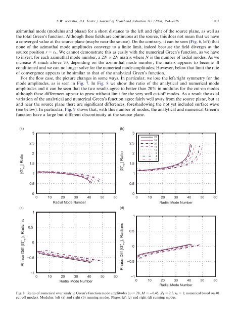
For the flow case, the picture changes in some ways. In particular, we lose the left/right symmetry for the
mode amplitudes, as is seen in Fig. 7. InFig. 8 we show the ratio of the analytical and numerical mode
amplitudes and it can be seen that the two results agree to better than 20% in modulus for the cut-on modes
although these differences appear to grow without limit for the very well cut-off modes. As a result the axial
variation of the analytical and numerical Green’s function agree fairly well away from the source plane, but at
and near the source plane there are significant differences, foreshadowing the not yet included surface wave
(see below). In particular, Fig. 9 shows that, with this number of modes, the analytical and numerical Green’s
function have a large but different discontinuity at the source plane.
|G −
| Ratio
mµ
Phase Diff (G −
), Radians
mµ
3
2.5
2
1.5
1
0.5
0.5
0
0 10 20 30 40 50 60
1
0
−0.5
S.W. Rienstra, B.J. Tester / Journal of Sound and Vibration 317 (2008) 994–1016 1007
Radial Mode Number
−1
0 10 20 30 40 50 60
Radial Mode Number
|G +
| Ratio
mµ
Phase Diff (G −+
), Radians
mµ
3
2.5
2
1.5
1
0.5
−0.5
0
0 10 20 30 40 50 60
1
0.5
0
28
24
20
16
12
8
4
0
Radial Mode Number
−1
0 10 20 30 40 50 60
Radial Mode Number
Fig. 8. Ratio of numerical over analytic Green’s function mode amplitudes (o ¼ 28, M ¼ 0:45, Z1 ¼ 2:5, r0 ¼ 1; numerical based on 40
cut-off modes). Modulus: left (a) and right (b) running modes. Phase: left (c) and right (d) running modes.