An analytic Green's function for a lined circular duct containing ...

ARTICLE IN PRESS
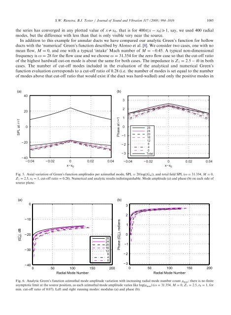
the series has converged in any plotted value of xax0, that is for 400pjx x0jb1, say, we used 400 radial
modes, but the difference with less than that is only visible very near the source.
In addition to this example for annular ducts we have compared our analytic Green’s function for hollow
ducts with the ‘numerical’ Green’s function described by Alonso et al. [8]. We consider two cases, one with no
mean flow, M ¼ 0, and one with a typical ‘intake’ Mach number of M ¼ 0:45. A typical non-dimensional
frequency is o ¼ 28 for the flow case and we choose o ¼ 31:354 for the zero flow case so that the cut-off ratio
of the highest hardwall cut-on mode is about the same for both cases. The impedance is Z1 ¼ 2:5 i0 in both
cases. The number of cut-off modes included in the evaluation of the analytical and numerical Green’s
function evaluation corresponds to a cut-off ratio of 0.28 (i.e. the number of modes is set equal to the number
of modes above that cut-off ratio that would exist if the duct was hard-walled) and only the positive modes in
SPL at r=1
40
20
0
−20
−40
−0.04 −0.02 0
x−x0 0.02 0.04
Phase at r=1
3
2
1
0
−1
−2
−3
28
24
20
16
12
8
4
0
Total
−0.04 −0.02 0
x−x0 0.02 0.04
Fig. 5. Axial variation of Green’s function amplitudes per azimuthal mode, SPL ¼ 20 logðjGmjÞ, and total field SPL (o ¼ 31:354, M ¼ 0,
Z1 ¼ 2:5, r0 ¼ 1, cut-off ratio ¼ 0:28). Numerical and analytic results indistinguishable. Mode amplitude (a) and phase (b) on each side of
source plane.
±
|Gm |, dB
0
−10
S.W. Rienstra, B.J. Tester / Journal of Sound and Vibration 317 (2008) 994–1016 1005
−20
−30
−40
28
24
20
16
12
8
4
0
0 50 100
Radial Mode Number
150 200
Phase (G± m ), radians
3
2
1
0
−1
−2
−3
0 50 100
Radial Mode Number
150 200
Fig. 6. Analytic Green’s function azimuthal mode amplitude variation with increasing radial mode number count m max; there is no finite
asymptotic limit at the source position, as each azimuthal mode amplitude varies like logðm maxÞ (o ¼ 31:354, M ¼ 0, Z1 ¼ 2:5, r0 ¼ 1, for
min. cut-off ratio of 0.07). Left and right running modes: modulus (a) and phase (b).