An analytic Green's function for a lined circular duct containing ...

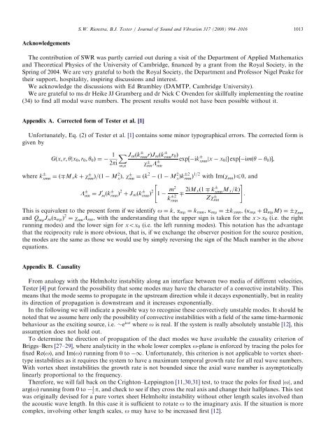
Acknowledgements
The contribution of SWR was partly carried out during a visit of the Department of Applied Mathematics
and Theoretical Physics of the University of Cambridge, financed by a grant from the Royal Society, in the
Spring of 2004. We are very grateful to both the Royal Society, the Department and Professor Nigel Peake for
their support, hospitality, inspiring discussions and interest.
We acknowledge the discussions with Ed Brambley (DAMTP, Cambridge University).
We are grateful to ms dr Heike JJ Gramberg and dr Nick C Ovenden for skillfully implementing the routine
(34) to find all modal wave numbers. The present results would not have been possible without it.
Appendix A. Corrected form of Tester et al. [1]
Unfortunately, Eq. (2) of Tester et al. [1] contains some minor typographical errors. The corrected form is
given by
Gðx; r; yjx0; r0; y0Þ ¼
1
2pi
X
m;n
JmðkrmnrÞJmðk rmnr0Þ exp½ ikxmnjx x0jŠ exp½ imðy y0ÞŠ,
wmnLmn where kxmn ¼ð Mxk þ wmnÞ=ð1 M2 xÞ, wmn ¼ðk2 ð1 M2 x rmnÞ1=2 with ImðwmnÞp0, and
Lmn ¼ J 0 mðkrmnÞ2 þ JmðkrmnÞ 2 1 m2
" #
2iMxð1 kxmnMx=kÞ .
Zwmn This is equivalent to the present form if we identify o ¼ k, amm ¼ krmn, kmm ¼ kxmn, ðkmm þ OmmMÞ ¼ w mn
and Q mmJmðammÞ 2 ¼ w mnLmn, with the understanding that the upper sign is taken for the x4x0 (i.e. the right
running modes) and the lower sign for xox0 (i.e. the left running modes). This notation has the advantage
that the reciprocity rule is more obvious, that is, if we exchange the observer position for the source position,
the modes are the same as those we would use by simply reversing the sign of the Mach number in the above
equations.
Appendix B. Causality
ARTICLE IN PRESS
S.W. Rienstra, B.J. Tester / Journal of Sound and Vibration 317 (2008) 994–1016 1013
From analogy with the Helmholtz instability along an interface between two media of different velocities,
Tester [4] put forward the possibility that some modes may have the character of a convective instability. This
means that the mode seems to propagate in the upstream direction while it decays exponentially, but in reality
its direction of propagation is downstream and it increases exponentially.
In the following we will indicate a possible way to recognise these convectively unstable modes. It should be
noted that we assume here only the possibility of convective instabilities with a field of the same time-harmonic
behaviour as the exciting source, i.e. eiot where o is real. If the system is really absolutely unstable [12], this
assumption does not hold out.
To determine the direction of propagation of the duct modes we have available the causality criterion of
Briggs–Bers [27–29], where analyticity in the whole lower complex o-plane is enforced by tracing the poles for
fixed ReðoÞ, andImðoÞrunning from 0 to 1. Unfortunately, this criterion is not applicable to vortex sheettype
instabilities as it requires the system to have a maximum temporal growth rate for all real wave numbers.
With vortex sheet instabilities the growth rate is not bounded since the axial wave number is asymptotically
linearly proportional to the frequency.
Therefore, we will fall back on the Crighton–Leppington [11,30,31] test, to trace the poles for fixed joj, and
argðoÞ running from 0 to 1
2 p, and check to see if they cross the real axis and change their halfplanes. This test
was originally devised for a pure vortex sheet Helmholtz instability without other length scales involved than
the acoustic wave length. In this case it is sufficient to rotate o to the imaginary axis. If the situation is more
complex, involving other length scales, o may have to be increased first [12].
k 2
rmn
Þk 2