An analytic Green's function for a lined circular duct containing ...

ARTICLE IN PRESS
Finally in order to show the behaviour of the analytical and numerical Green’s function continuity at the
source plane away from the source position, Fig. 12 for the zero flow case, shows the variation in the radial
direction at the source plane, at the same azimuthal angle as the source, of the modulus of the azimuthal mode
number amplitudes and also the total field, in dB. Shown for comparison is the free-field Green’s function
1=ð4pRÞ, where R is the distance from the source at r0 ¼ 1, multiplied by a plane wave correction to account
for the reflection or image source in the lined duct wall equal to 2Z1=ðZ1 þ 1Þ. It can be seen that the
agreement between the analytical and corrected free-field Green’s function for this zero flow case is very good
and that continuity (i.e. the total field made up of right running modes ðþÞ equals the total field made up of
left running modes ð Þ) at the source plane is achieved away from the source position—these are
indistinguishable for this zero flow case. Here we have decreased the cut-off ratio to 0.07 for the analytic
Green’s function evaluation but had to limit the numerical Green’s function evaluation to 40 cut-off radial
modes to avoid serious corruption of the solution due to ill-conditioned matrices for the higher azimuthal
modes.
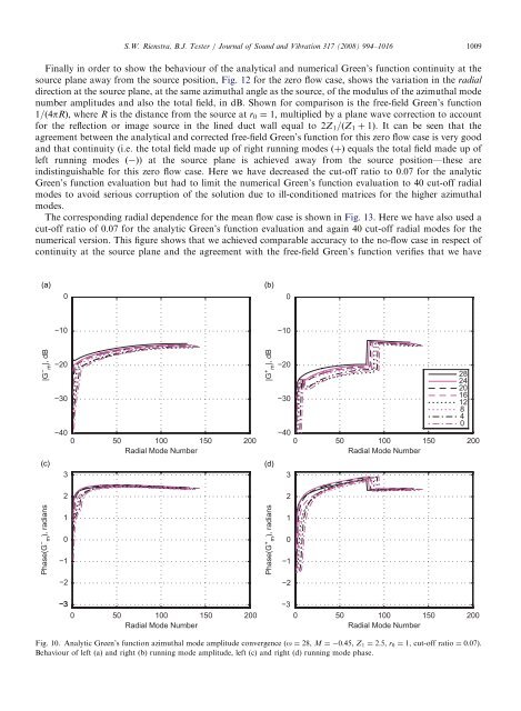
The corresponding radial dependence for the mean flow case is shown in Fig. 13. Here we have also used a
cut-off ratio of 0.07 for the analytic Green’s function evaluation and again 40 cut-off radial modes for the
numerical version. This figure shows that we achieved comparable accuracy to the no-flow case in respect of
continuity at the source plane and the agreement with the free-field Green’s function verifies that we have
|G− m |, dB
Phase(G− m ), radians
0
−10
−20
−30
−40
0 50 100
Radial Mode Number
150 200
3
2
1
0
−1
−2
S.W. Rienstra, B.J. Tester / Journal of Sound and Vibration 317 (2008) 994–1016 1009
−3
0 50 100
Radial Mode Number
150 200
|G + m |, dB
Phase(G + m ), radians
0
−10
−20
−30
−40
28
24
20
16
12
8
4
0
0 50 100
Radial Mode Number
150 200
3
2
1
0
−1
−2
−3
0 50 100
Radial Mode Number
150 200
Fig. 10. Analytic Green’s function azimuthal mode amplitude convergence (o ¼ 28, M ¼ 0:45, Z1 ¼ 2:5, r0 ¼ 1, cut-off ratio ¼ 0:07).
Behaviour of left (a) and right (b) running mode amplitude, left (c) and right (d) running mode phase.