Wall Pressure and Shear Stress Spectra from Direct Numerical ...
Wall Pressure and Shear Stress Spectra from Direct Numerical ...
Wall Pressure and Shear Stress Spectra from Direct Numerical ...

Create successful ePaper yourself
Turn your PDF publications into a flip-book with our unique Google optimized e-Paper software.
6 HU, MORFEY, AND SANDHAM<br />
the periodically specified computational box is equal to<br />
! 2 f =u 2 2 U c=L xRe 0:02. In the simulation both<br />
the fundamental frequency <strong>and</strong> its first harmonic appeared in the<br />
spectrum. This value equals 0.029 for the 130 case, where a much<br />
less pronounced peak is also observed in the spectrum. This<br />
phenomenon only occurs at low Reynolds number when turbulence<br />
exhibits a self-generation mechanism as has been found by Jimenez<br />
<strong>and</strong> Moin [30] <strong>and</strong> Hamilton et al. [31]. As large computational<br />
boxes (L x 48 for Re 90 <strong>and</strong> L x 24 for Re 130) were used<br />
for these simulations, the peaks appear at low frequencies, <strong>and</strong><br />
contribute little to the rms pressure. For example, replacing the<br />
values in the Re 90 spectrum for the points within the two peaks<br />
(3 points for the first peak <strong>and</strong> 7 points for the second) with linearly<br />
interpolated values <strong>from</strong> neighboring points brings the calculated<br />
rms wall pressure down <strong>from</strong> 1.14 to 1.10.<br />
Figure 5 compares DNS data with measurements of wall-pressure<br />
spectra by Brungart et al. [4] for channel flow at Re 1120, by<br />
Lauchle <strong>and</strong> Daniels [25] for fully developed pipe flow at<br />
Re 1400, <strong>and</strong> by Schewe [1] for a boundary layer in<br />
nonaccelerating flow at Re 1400. The current DNS cases have<br />
Reynolds numbers Re (based on channel centerline velocity <strong>and</strong><br />
momentum thickness) that range <strong>from</strong> 142 to 2959. It can be seen that<br />
DNS data for Re 720 (plotted as a dashed line in the figure, with<br />
Re 1343) compare well with the experimental data of Brungart<br />
et al. [4] <strong>and</strong> Schewe [1], but are higher especially at low frequency<br />
than the pipe flow data of Lauchle <strong>and</strong> Daniels [25]. A similar<br />
comparison was also presented in Fig. 11 of Hu et al. [14]; a<br />
correction factor of 8=3 should be applied to the three DNS cases<br />
(Re 360, 180, <strong>and</strong> 90) plotted in that figure.<br />
The rms fluctuating wall pressure p rms w scaled by mean wall<br />
shear stress w is plotted in Fig. 6 for the DNS cases listed in Table 1.<br />
The current data are consistent with the DNS results for channel flow<br />
of KMM [9] <strong>and</strong> MKM [10]. Experimental data <strong>from</strong> Farabee <strong>and</strong><br />
Casarella [2], Lauchle <strong>and</strong> Daniels [25], Schewe [1], <strong>and</strong> Bull <strong>and</strong><br />
Thomas [32] are also plotted for comparison. Our present DNS<br />
results fall within the scatter of the experimental data. Farabee <strong>and</strong><br />
Casarella [2] concluded that the mean square wall-pressure<br />
fluctuation varies linearly with the logarithm of Reynolds number. A<br />
best fit to the current results <strong>and</strong> the DNS data of Moser [10] for<br />
Re 360 gives the following formula, shown in Fig. 6 by a solid<br />
line:<br />
p rms 2 w 2:60 ln Re 11:25 (8)<br />
The slope is steeper than that given by Farabee <strong>and</strong> Casarella [2],<br />
which is shown by a dash-dotted line in Fig. 5.<br />
(p rms ) w<br />
4<br />
3<br />
2<br />
1<br />
♦<br />
♦<br />
♦<br />
♦<br />
♦<br />
♦ ⋅ ⋅⋅⋅⋅⋅<br />
10<br />
Reτ 2<br />
10 3<br />
0<br />
Fig. 6 DNS results of rms wall pressure (⧫) compared with DNS of<br />
KMM [9] (r) <strong>and</strong> MKM [10] ( ), <strong>and</strong> with experiments of Farabee <strong>and</strong><br />
Casarella [2] ( ), Lauchle <strong>and</strong> Daniels [25] (▷), Schewe [32] ( ), <strong>and</strong> Bull<br />
<strong>and</strong> Thomas [32] (□). Solid line: best fit of DNS data, Eq. (8); dash-dotted<br />
line: formula of Farabee <strong>and</strong> Casarella [2].<br />
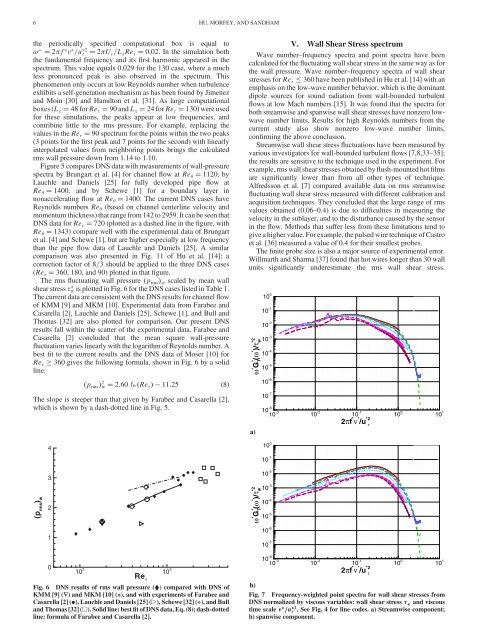
V. <strong>Wall</strong> <strong>Shear</strong> <strong>Stress</strong> spectrum<br />
Wave number–frequency spectra <strong>and</strong> point spectra have been<br />
calculated for the fluctuating wall shear stress in the same way as for<br />
the wall pressure. Wave number–frequency spectra of wall shear<br />
stresses for Re 360 have been published in Hu et al. [14] with an<br />
emphasis on the low-wave number behavior, which is the dominant<br />
dipole sources for sound radiation <strong>from</strong> wall-bounded turbulent<br />
flows at low Mach numbers [15]. It was found that the spectra for<br />
both streamwise <strong>and</strong> spanwise wall shear stresses have nonzero lowwave<br />
number limits. Results for high Reynolds numbers <strong>from</strong> the<br />
current study also show nonzero low-wave number limits,<br />
confirming the above conclusion.<br />
Streamwise wall shear stress fluctuations have been measured by<br />
various investigators for wall-bounded turbulent flows [7,8,33–35];<br />
the results are sensitive to the technique used in the experiment. For<br />
example, rms wall shear stresses obtained by flush-mounted hot films<br />
are significantly lower than <strong>from</strong> all other types of technique.<br />
Alfredsson et al. [7] compared available data on rms streamwise<br />
fluctuating wall shear stress measured with different calibration <strong>and</strong><br />
acquisition techniques. They concluded that the large range of rms<br />
values obtained (0.06–0.4) is due to difficulties in measuring the<br />
velocity in the sublayer, <strong>and</strong> to the disturbance caused by the sensor<br />
in the flow. Methods that suffer less <strong>from</strong> these limitations tend to<br />
give a higher value. For example, the pulsed wire technique of Castro<br />
et al. [36] measured a value of 0.4 for their smallest probes.<br />
The finite probe size is also a major source of experimental error.<br />
Willmarth <strong>and</strong> Sharma [37] found that hot wires longer than 30 wall<br />
units significantly underestimate the rms wall shear stress.<br />
ω * * * *2<br />
G (ω )/τw<br />
T<br />
a)<br />
* * *2<br />
(ω )/τw<br />
ω * G T<br />
10 0<br />
10 -1<br />
10 -2<br />
10 -3<br />
10 -4<br />
10 -5<br />
10 -6<br />
10 -7<br />
10 -3 10 -8<br />
10 0<br />
10 -1<br />
10 -2<br />
10 -3<br />
10 -4<br />
10 -5<br />
10 -6<br />
10 -7<br />
10 -3 10 -8<br />
10 -2<br />
10 -2<br />
2πf * ν * /u *2<br />
10<br />
τ<br />
-1<br />
2πf * ν * /u *2<br />
10<br />
τ<br />
-1<br />
b)<br />
Fig. 7 Frequency-weighted point spectra for wall shear stresses <strong>from</strong><br />
DNS normalized by viscous variables: wall shear stress w <strong>and</strong> viscous<br />
time scale =u 2 . See Fig. 4 for line codes. a) Streamwise component;<br />
b) spanwise component.<br />
10 0<br />
10 0<br />
10 1<br />
10 1