Wall Pressure and Shear Stress Spectra from Direct Numerical ...

4 HU, MORFEY, AND SANDHAM
Loss Gain
0.3
0.2
0.1
0
-0.1
-0.2
z +
10 -2
10 -1
10 0
10 1
10 2
10 3
-0.3
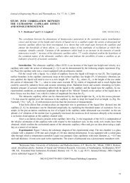
Fig. 3 Turbulent kinetic energy budget for Re 1440. All quantities
are scaled by u 4 = .
of samples N is even.
The two-sided wave number–frequency spectrum for wall
pressure or wall shear stresses, S q k xl;k ym;f s ,isdefined as the
following mathematical expectation, averaged over a large box
(L x L y) and a long sample (duration T N t):
S q k xl;k ym;f s E lim
L x;L y;T!1
0.0005
^q ^q ?
2 2 L xL yT
The factor of 2 2 is due to the use of wave number components kx,
k y rather than spatial frequencies. It should be mentioned that the sign
convention used here for time Fourier transformation differs from the
usual mathematical convention. The time transform is defined so that
waves with the same sign of streamwise wave number and frequency
travel with the flow, and waves with opposite signs travel against the
flow.
To improve the quality of the spectral estimates, the time record is
split into N seg time segments with 50% overlap. Wave number–
frequency spectra are calculated for each time segment and averaged
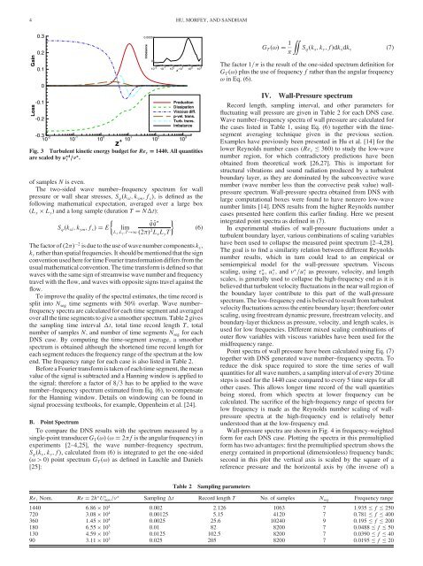
over all the time segments to give a smoother spectrum. Table 2 gives
the sampling time interval t, total time record length T, total
number of samples N, and number of time segments N seg for each
DNS case. By computing the time-segment average, a smoother
spectrum is obtained although the shortened time record length for
each segment reduces the frequency range of the spectrum at the low
end. The frequency range for each case is also listed in Table 2.
Before a Fourier transform is taken of each time segment, the mean
value of the signal is subtracted and a Hanning window is applied to
the signal; therefore a factor of 8=3 has to be applied to the wave
number–frequency spectrum estimated from Eq. (6), to compensate
for the Hanning window. Details on windowing can be found in
signal processing textbooks, for example, Oppenheim et al. [24].
B. Point Spectrum
To compare the DNS results with the spectrum measured by a
single-point transducer G T ! (! 2 f is the angular frequency) in
experiments [2–4,25], the wave number–frequency spectrum,
S q k x;k y;f , calculated from (6) is integrated to get the one-sided
(!>0) point spectrum G T ! as defined in Lauchle and Daniels
[25]:
Imbalance
0
z +
10 -2 10 -1
10 0
10 1
10 2
10 3
Production
Dissipation
Viscous diff.
p-vel. trans.
Turb. trans.
Imbalance
(6)
Table 2 Sampling parameters
G T !
1 ZZ
S q k x;k y;f dk xdk y
The factor 1= is the result of the one-sided spectrum definition for
G T ! plus the use of frequency f rather than the angular frequency
! in Eq. (6).
IV. Wall-Pressure spectrum
Record length, sampling interval, and other parameters for
fluctuating wall pressure are given in Table 2 for each DNS case.
Wave number–frequency spectra of wall pressure are calculated for
the cases listed in Table 1, using Eq. (6) together with the timesegment
averaging technique given in the previous section.
Examples have previously been presented in Hu et al. [14] for the
lower Reynolds number cases (Re 360) to study the low-wave
number region, for which contradictory predictions have been
obtained from theoretical work [26,27]. This is important for
structural vibrations and sound radiation produced by a turbulent
boundary layer, as they are dominated by the subconvective wave
number (wave number less than the convective peak value) wallpressure
spectrum. Wall-pressure spectra obtained from DNS with
large computational boxes were found to have nonzero low-wave
number limits [14]. DNS results from the higher Reynolds number
cases presented here confirm this earlier finding. Here we present
integrated point spectra as defined in (7).
In experimental studies of wall-pressure fluctuations under a
turbulent boundary layer, various combinations of scaling variables
have been used to collapse the measured point spectrum [2–4,28].
The goal is to find a similarity relation between different Reynolds
number results, which in turn could lead to an empirical or
semiempirical model for the wall-pressure spectrum. Viscous
scaling, using w, u , and =u as pressure, velocity, and length
scales, is generally used to collapse the high-frequency end as it is
believed that turbulent velocity fluctuations in the near wall region of
the boundary layer contribute to this part of the wall-pressure
spectrum. The low-frequency end is believed to result from turbulent
velocity fluctuations across the entire boundary layer; therefore outer
scaling, using freestream dynamic pressure, freestream velocity, and
boundary-layer thickness as pressure, velocity, and length scales, is
used for low frequencies. Different mixed scaling combinations of
outer flow variables with viscous variables have been used for the
midfrequency range.
Point spectra of wall pressure have been calculated using Eq. (7)
together with DNS generated wave number–frequency spectra. To
reduce the disk space required to store the time series of wall
quantities for all wave numbers, a sampling interval of every 20 time
steps is used for the 1440 case compared to every 5 time steps for all
other cases. This allows longer time record of the wall quantities
being stored, from which spectra at lower frequency can be
calculated. The sacrifice of the high-frequency range of spectra for
low frequency is made as the Reynolds number scaling of wallpressure
spectra at the high-frequency end is relatively better
understood than at the low-frequency end.
Wall-pressure spectra are shown in Fig. 4 in frequency-weighted
form for each DNS case. Plotting the spectra in this premultiplied
form has two advantages: first the premultiplied spectrum shows the
energy contained in proportional (dimensionless) frequency bands;
second in this plot the vertical axis is scaled by the square of a
reference pressure and the horizontal axis by (the inverse of) a
Re Nom. Re 2h Umax= Sampling t Record length T No. of samples Nseg Frequency range
1440 6:86 104 0.002 2.126 1063 7 1:935 f 250
720 3:08 104 0.00125 5.15 4120 7 0:781 f 400
360 1:45 104 0.0025 25.6 10240 9 0:195 f 200
180 6:55 103 0.01 82 8200 7 0:0488 f 50
130 4:59 103 0.0125 102.5 8200 7 0:0390 f 40
90 3:11 103 0.025 205 8200 7 0:0195 f 20
(7)