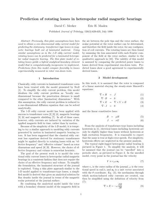
Prediction of rotating losses in heteropolar radial magnetic bearings

Prediction of rotating losses in heteropolar radial magnetic bearings
Abstract: Previously, thin plate assumptions have been
used to obtain a one-dimensional eddy current model for
predicting the stationary, transformer-type losses in magnetic
bearings built out of laminated material. Using
similar assumptions as in the 1-D eddy current model,
rotating losses can be predicted for a laminated heteropolar
radial magnetic bearing. The thin plate model of rotating
losses yields a hybrid analytical-boundary element
model that is computationally inexpensive to implement.
Predictions from this model compare favorably to losses
experimentally measured in rotor run-down tests.
1 Introduction
Classically, eddy currents in laminated transformer cores
have been treated with the model presented by Stoll
[1]. To simplify the eddy current problem, this model
idealizes the eddy current problem as “locally onedimensional
because the penetration distance is small
compared to the other [lamination] dimensions.” With
this assumption, the eddy current problem is reduced to
a one-dimensional diffusion equation that can be solved
analytically.
The 1-D eddy current model has been applied with
success to transformer cores [2] [3] [4], magnetic bearings
[5] [6] and magnetic shielding [7]. In all of these cases,
however, eddy currents are induced by variation of the
applied magnetic field in time, rather than by motion.
Because of the simplicity of the 1-D model, it is tempting
to try a similar approach to modeling eddy currents
generated by motion in laminated magnetic bearing rotors.
It has been suggested that the classical eddy current
loss equations derived for stationary transformers
might be applied directly to rotating losses with an “effective
frequency” and “effective volume” based on rotor
dimensions and speed [8] [9]. However, the choice of effective
frequency and volume is somewhat heuristic.
The goal of the present work is to model the rotational
eddy current losses in heteropolar radial magnetic
bearings in a consistent fashion that does not require the
choice of an effective frequency and volume. To simplify
the formulation, the laminated structure of the journal
is exploited. Using a thin plate approach similar to the
1-D model applied to transformer-type losses, a simplified
model is derived that gives an analytical solution for
flux density inside the journal in terms of the magnetic
scalar potential at the journal surface.
By combining the analytical model inside the rotor
with a boundary element model of the magnetic field in
David C. Meeker Eric H. Maslen
Published Journal of Tribology, 120(3):629-635, July 1998
1
theairbetweenthepoletipsandtherotorsurface,the
scalar potential at the rotor surface can be determined,
and therefore the field inside the rotor, for any configuration
of coil currents. The rotating losses are then found
by summing the loss associated with each Fourier component
of the field at the rotor surface, similar to the
qualitative approach in [10]. The validity of this model
is assessed by comparing the predicted power losses to
losses derived from experimental run-down tests. Predicted
losses show a good agreement to experimentally
derived losses.
2 Model development
In this work, it is assumed that the rotor is composed
of a linear material obeying the steady-state Maxwell’s
equations:
∇×H = J (1)
∇·B = 0 (2)
∇×E = ∇×V × B (3)
∇·J = 0 (4)
and the linear constitutive laws:
B = µH (5)
J = σE (6)
From the analysis of transformer-type losses including
hysteresis in [1], electrical losses including hysteresis are
only be slightly higher than losses without hysteresis at
high excitation frequencies. It is reasonable to expect
that the same is true at high rotor speeds. For simplicity,
hysteresis effects are neglected in the present analysis.
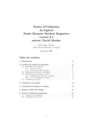
The typical eight-legged heteropolar radial bearing is
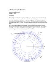
pictured in Figure 1. To simplify the analysis, it will
be assumed that the journal can be “unrolled” into a
periodic sheet, as pictured in Figure 2. In the unrolled
model, every point in the journal has the velocity
V ≡ roω a2
(7)
where ro is the outer radius of the journal, ω is the rotational
speed in rad/s, and a2 is a unit vector associated
with the θ coordinate. Eq. (3), the mechanism through
which motion-induced eddy currents are created, can
then be simplified using the definition of velocity from
(7):
∇×E = −ω ∂B
(8)
∂θ

stator
journal
Figure 1: Typical eight legged heteropolar bearing.
8
7
6
stator poles
5
journal
4
3
2
θ , a 2
Figure 2: “Unrolled” heteropolar bearing.
1
r, a 1
z, a 3
A partial differential equation describing the flux distribution
inside one lamination is derived by first taking
the curl of (1):
∇×∇×H = ∇×J (9)
Then, the constitutive laws are used to write (9) in terms
of B and E:
∇×∇×B = σµo ∇×E (10)
Applying equation (2) to (10) to enforce the zero divergence
of B yields:
−∇ 2 B = σµo ∇×E (11)
Finally, (8) is substituted into (11) to give the differential
equation describing the flux density inside each lamination:
∇ 2 B = ωσµ ∂B
∂θ
(12)
No thin-plate assumption has yet been made.
unrolled domain,
In the
∇ 2 ≡ ∂2 1
+
∂r2 r2 ∂
o
2
∂2
+
∂θ2 ∂z2 (13)
If the rotor is composed of thin laminations in the a3
direction, the cross-lamination second-order term ∂2
∂z2 can be expected to dominate ∇2 r,θB because the second
derivatives of B with respect to z must be huge to affect
any change B across the lamination thickness. The
thin-plate model assumes that the r and θ second-order
2
d
θ
Figure 3: Detailed view of a single rotor lamination.
components are so insignificant compared to the z component
that they can be neglected altogether. Applying
the thin-plate assumption to (12) yields a simplified eddy
current model driven by journal motion:
∂2B ∂B
= ωσµ
∂z2 ∂θ
r
z
(14)
Equation (14) is very similar to Stoll’s 1-D diffusion
equation; the difference is that for transformer-type
losses, the first-order derivative on the right-hand side
is with respect to time rather than the spatial coordinate
θ.
Since the unrolled domain is 2π periodic in the θ coordinate,
the solution for B is expected to consist of harmonics
in θ. A phasor representation [11] can be adopted
where B is understood to be the real part of
∞
bn e jnθ ∞
≡ bn (cos nθ + jsinnθ) (15)
n=0
n=0
where bn is a complex number denoting the magnitude
and phase of the n th harmonic component of B. Since
the system is linear, each harmonic can be considered
separately and the results for all harmonics superimposed
to yield a solution for B.
Substituting the phasor representation for B into (14)
yields
∂ 2 bn
∂z 2 ejnθ = jnωσµbn e jnθ
Each side can be divided by e jnθ :
(16)
∂ 2 bn
∂z 2 = jnωσµbn (17)
In the phasor representation, the flux distribution for
each harmonic is merely an ordinary differential equation
respect to z, the coordinate in the plate thickness
direction.
Boundary conditions must be specified if (17) is to be
solved for the flux distribution in the laminated rotor.
Let each lamination be of thickness d, and let the z =0
at the center of the lamination of interest, as illustrated
in Figure 3. Since the model is pseudo-2-dimensional
(that is, the flux density distribution is the same in every
lamination in the journal), one would expect no a3

component of bn at the interface between laminations.
The axial component of B, bn · a3, is therefore equal to
zero everywhere. The a1 and a2 boundary condition at
interface between laminations then specified as
B[r, θ, d
2 ]=Bo[r, θ];
∂B
[r, θ, 0] = 0 (18)
∂z
where Bo[r, θ] is some unknown function of r and θ that
is yet to be determined. Converting the boundary conditions
into the phasor representation gives:
bn[r, d/2] = bn,o[r];
∂bn
[r, 0] = 0
∂z
(19)
where bn,o represents the nth harmonic component of
Bo. Equation (17) subject to (19) is the same equation
that must be solved in [1]for transformer-type losses; the
solution is
bn[r, z] =bn,o[r] cosh[√ jnωσµz]
cosh[ √ jnωσµ d
2 ]
(20)
The average flux density, ¯ bn, at in the lamination is found
by integrating across the lamination:
¯ bn = 2
d
= bn,o
d/2
bn[r, z] dz (21)
o
tanh[ √ jnωσµ d
2 ]
√ d jnωσµ 2
However, the boundary field distribution, bn,o, hasnot
yet been determined in the a1 and a2 directions. This
boundary condition should be chosen such that zero divergence
of B, equation (2), is satisfied. To solve for an
appropriate Bo, define magnetic scalar potential Ω as
−µ ∇Ω =Bo
(22)
Since there is no a3 component of B, zero divergence is
satisfied if
∇r,θ · Bo = 0 (23)
The zero divergence of Bo written in terms of scalar potential
is
∇ 2 Ω = 0 (24)
Transforming (24) into the phasor representation yields:
∂2 2 Ωn n
− Ωn = 0 (25)
∂r2 ro
It is reasonable to impose the boundary condition
∂Ωn
∂r =0; r = ri (26)
which requires that no flux crosses the inner radius of
the journal at r = ri. Atr = ro, the outer radius of the
journal, the value of Ωn is some specified value, Ωn,o:
Ωn[ro] =Ωn,o
(27)
Solving (25) with these boundary conditions gives the
scalar potential for each harmonic in terms of scalar potential
at the journal surface:
Ωn[r] =Ωn,o
cosh[ n (r − ri)]
ro
cosh[ n
ro (ro − ri)]
(28)
Eqs. (20) and (28) are combined to describe each harmonic
of flux density in the journal:
n
bn = −µ Ωn,o
ro
cosh[ √ jnωσµz]
cosh[ √ jnωσµ d
2 ]
∗ (29)
n sinh[ (r − ri)]
ro
cosh[ n
ro (ro − ri)] a1
n cosh[ (r − ri)]
ro + j
cosh[ n
ro (ro − ri)] a2
Through (29), the flux density is defined in terms of
unknown Fourier series coefficients of the magnetic scalar
potential at the rotor surface. If an input-output relationship
between applied potential at the rotor surface
to resulting flux passing normal to the rotor surface is
formed, the analytical solution for the field inside the
journal can be combined with a computational model of
the rest of the bearing to determine the unknown distribution
Ωo[θ] at the rotor surface.
To simplify the analysis, it will be assumed that the
flux in the gap is purely 2-dimensional. However, the
solution in the lamination is a function of z, ascanbe
seen in (20). It will be assumed that a transition between
the 2-d solution in the gap and the fully-developed profile
described by (20) takes place in a very thin skin region
near the surface of the rotor. The interface with the air
is then modeled by a conservation of flux passing normal
to the air-iron interface:
or for each harmonic:
(air) (B · a1) = (iron) ( ¯ B · a1) (30)
(air) (bn · a1) = (iron) ( ¯ bn · a1) (31)
In terms of scalar potential, the conservation condition
is
∂
√ d
(air)Ωn µ tanh[ jnωσµ 2
µo
=
∂r
]
∂
(iron)Ωn
√ d jnωσµ ∂r
2
(32)
For continuity of H on the air-iron boundary,
(air) Ωn = (iron) Ωn
(33)
By differentiating (28) with respect to r, and substituting
into (32), a boundary condition results that relates the
applied scalar potential on the journal surface, Ωn, toits
normal derivative on the air side of the iron-air interface:
∂Ωn n = µr( ro ∂r )
√ d
tanh[ jnωσµ 2 ]
√ tanh[ d jnωσµ 2
n
ro (ro − ri)] Ωn
(34)
3

This expression can be re-arranged into real and imaginary
parts as
where
Gr = µr
∂Ωn
∂r =(Gr + jGi)Ωn (35)
nδn
ro d
sin d
d +sinh δn δn
cos d
d +cosh δn δn
n tanh ro (ro
− ri)
(36)
nδn
Gi = µr
ro d
sin d
d − sinh δn δn
cos d
n tanh
d
ro +cosh δn δn
(ro
− ri)
(37)
and
1
2 2
δn =
(38)
nωσµ
is the skin depth associated with each harmonic. Eq.
(34) specifies the relationship between potential in the
air to the normal gradient of potential at the surface of
the rotor. By solving for the potential distribution in the
in the air only subject to boundary condition (34), the
field inside the rotor is uniquely specified by (29).
3 Power loss
If the magnetic scalar potential is known at the rotor
surface, the field distribution in the journal is known,
and eddy current power losses can be computed. This
loss, P , is found by integrating resistive power loss over
the volume of the rotor:
P =
ro
ri
d
2
− d
2
2π
0
1
J · Jrodz dr dθ (39)
σ
Current density J is found via (1), by taking the curl of
the field intensity. Since the r and θ variation of H are
described by scalar potential Ω, J · J simplifies consider-
ably to
J · J =
2 ∂H1
+
∂z
2 ∂H2
∂z
(40)
By orthogonality of sines and cosines, cross-products
between different harmonics integrate to zero when (40)
is evaluated over the entire volume of the journal. The
power loss contributions from each harmonic can be considered
separately and the results summed to get the total
motion-induced power loss:
P =
∞
n=0
Pn
For each harmonic, the power loss is
Pn = πro
σµ
ro
ri
d
2
− d
2
∂bn
∂z
2
(41)
dz dr (42)
4
d Ω/ dr = 0
d Ω/ dr = 0
journal
apply (31)
Ω= N i
3
air
ω
Ω = N i
2
Ω=
N i
1
Figure 4: Simplified computational domain for modeling
fringing effects.
where ∂bn
∂z is found by differentiating (29) with respect
to z. Integrating (42) yields:
Pn = |Ωn,o| 2
2πn
σδn
tanh[ n
ro (ro−ri)]
d d
sinh − sin δn δn
cosh d
δn
+cos d
δn
(43)
Equation (43) is the loss for each lamination; this loss
must be multiplied by the number of laminations in the
journal to get the total bearing losses.
4 Incorporation of the journal solution with
the bearing structure
If the field at the surface of the rotor is known, the rotating
power loss can be determined via (43). As noted by
Matsumura [10], the distribution of flux on the air-iron
boundary has a large influence on the resulting power
losses, and the motion-induced eddy currents somewhat
alter the field distribution from the zero speed form. To
determine the correct potential distribution at the surface
of the rotor, the analytical solution inside the rotor
must be coupled to a numerical solution for the field in
the air between the poles and rotor surface.
An elaborate finite element or boundary element
model could be used to represent the stator. For the
purposes of this study, however, a very elaborate model
is unnecessarily complicated. The goal is to model the
fringing of flux around the edges of the poles correctly.
To perform this task, it is sufficient to use the simple
computational domain pictured in Figure 4. The computational
domain is a thin annulus of air between the
rotor surface and pole tips.
If the stator is built of highly permeable material,
the stator back-iron can be considered magnetically
“grounded” at zero potential. The potential on a section
of the outside boundary of the annulus associated with
the k th pole can then be specified to be Nik, thenumber
of Amp-Turns of current flowing in the coil around the
k th pole.
Between pole tips, the boundary condition ∂Ω/∂r =0
is applied. This boundary condition forces all flux to

pass the outer boundary of the annulus through the pole
faces.
On the inside surface of the air annulus, boundary condition
(34) is applied. Equation (34) is a phasor relationship
between potential and its normal derivative on the
boundary; to apply a numerical method, this boundary
condition must be written in terms of spatial field values
at points on the boundary of the computational domain.
To apply the boundary condition, the spatial boundary
values must be transformed into the phasor representation,
the boundary conditions applied, and then transformed
back into spatial coordinates. The transformation
to phasor form is
Ωn,o = 1
2π
(Ωo[θ]cosnθ − j Ωo[θ]sinnθ) dθ ; n>0
π 0
(44)
Ω0,o = 1
2π
Ωo[θ] dθ (45)
2π 0
However, the boundary is represented by a finite number
of elements. Specifically, let the rotor surface be divided
into m discrete elements. Inside each element, the scalar
potential and normal gradient of scalar potential are approximated
with constant trial functions. Equations (44)
and (45) can then be approximated by the discrete transforms:
Ωn,o = 2
m
(Ωo[k]cos[nk δθ] − j Ωo[k]sin[nk δθ])
m
k=1
(46)
Ω0,o = 1
m
Ωo[k] (47)
m
k=1
where Ωo[k] is the value of scalar potential a the center of
the kth element, and δθ is the length of each element in
radians. Eqs. (46) and (47) are a linear transformation
between the spatial and phasor representations of Ω on
the rotor surface. Since there are only a finite number
of boundary elements, only the first m
2 harmonics can be
represented.
Since boundary condition (34) couples all boundary
nodal values, it is unsuitable for use with a finite element
scheme in which bandedness of the resulting stiffness
matrix is essential to an efficient solution. Instead,
a boundary element analysis is indicated. A boundary
element scheme trades a large but banded matrix for
a much smaller but full matrix. Applying a boundary
condition that couples together all boundary nodes is
consistent with the boundary element formulation. A
detailed description of the boundary method with constant
trial function elements applied to solving ∇2Ω=0 is contained in [12].
5 Comparison of model to experimentally
measured losses
5.1 Identification of materials properties
It is apparent from the inspection of (43) that the rotating
eddy current losses are strongly dependent on the
5
L R R
c s
v
Figure 5: Ring test circuit.
magnetic permeability, µ, and the electrical conductivity,
σ, of the journal material. These properties may
vary widely for a particular material depending upon
heat treatment. To get accurate materials properties to
use for the rotating loss model, these properties must be
accurately determined.
The desired materials properties can be obtained by
testing the frequency response of a test ring built from
the same batch of laminations from which the journal
was constructed. To perform the test, the laminated
test ring is wound with a number of turns of wire to
form a simple choke. A sinusoidal excitation of different
frequencies is applied across this winding. The timevarying
nature of the excitation induces eddy currents
in the test ring. From Stoll, the effect of these eddy
currents can be thought of as modifying the permeability
of the core material. Derived from a thin plate model, the
frequency-dependent permeability of the core material is:
Θ
Θ √
e− 2 − d
tanh[e 2 j ˆωσµ 2 µfd[jˆω] =µ ]
√ d j ˆωσµ 2
1
v
2
(48)
where ˆω is the frequency of excitation. In this expression,
the effects of hysteresis in the core material is idealized
as a pure phase lag between B and H of Θ radians.
Including the effects of eddy currents and hysteresis, the
frequency-dependent inductance of the coil is:
L[j ˆω] = N 2 aµfd[jˆω] (49)
πD
where N is the number of turns wound around the core,
a is the cross-sectional area, and D is the mean diameter
of the ring. The frequency response of the ring is tested
with the circuit pictured in Figure 5. The input is voltage
v1 is supplied across the coil and a sensing resistor, Rs.
The output is the voltage v2 across the sensing resistor,
which is proportional to current in the coil. The overall
transfer function of the test circuit is:
v2
v1
=
(50)
j ˆωL[jˆω]+Rc + Rs
Eddy currents and hysteresis cause a substantial deviation
in frequency response from what would be expected
in the absence of eddy currents. By fitting the permeability,
conductivity, and hysteresis angle so that (50)
Rs

V2/V1
degrees
0.7
0.5
0.3
20. 50. 100. 200. 500. 1000.
Model w/ eddy & hysteresis
Model w/ eddy only
Model w/out eddy or hyst.
Experiment
Hertz
Figure 6: Magnitude response of ring test circuit.
-20
-40
-60
20. 50. 100. 200. 500. 1000.
Model w/ eddy & hysteresis
Model w/ eddy only
Model w/out eddy or hyst.
Experiment
Hertz
Figure 7: Phase shift ring test circuit.
closely matches the measured response of the circuit, the
materials properties of the core material are identified.
This procedure was used to find the materials properties
of the high-speed test rig described by Kasarda et.
al [8]. A test ring was constructed out of 14 mil, 3%
silicon-iron laminations with and inner diameter of 2.54
cm, an outer diameter of 3.175 cm, and a length of 1.65
cm. The ring was tested at a number of frequencies between
10 and 1000 Hz. The coil and sense resistances
were measured as 0.50 Ω and 15.30 Ω respectively. Using
this data, the materials properties that provide a best
fit are: σ = 7.46(10 6 )(Ω − m) −1 , µ = 3460 µo, and
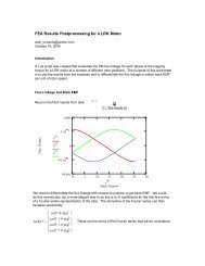
Θ=20 o . The magnitude and phase of the experiment
and fit are shown in Figures 6 and 7 respectively. For
comparison, the predicted response neglecting the effects
of eddy currents is also included, and the eddy currents
can be seen to have a pronounced effect on the response
of the circuit above 100 Hz. The model with eddy currents
and hysteresis shows a very good agreement in both
magnitude and phase with the test circuit. The agreement
with eddy currents but neglecting hysteresis effects
is also relatively good, but this model tends to predict
more phase lag than was actually observed. The fact that
the best fit is achieved by including hysteresis highlights
the need for the evental inclusion of hysteresis effects in
the rotating loss model.
6
5.2 Determination of electrical losses from rundown
data
The energy stored in the rotor at any time is
E = 1
2 Jω2
(51)
The change in energy with respect to time corresponds
to power loss, Ptot, due to eddy currents, hysteresis, and
windage:
Ptot = − dE
= −Jω˙ω (52)
dt
By measuring the rundown of a shaft in magnetic bearings,
the power loss at any speed can be found by substituting
the experimental data run-down into (52). However,
the loss of interest is not the total loss, but rather
the loss component due to magnetic effects. If it is assumed
that a linear magnetic model applies, eddy current
losses should scale with the square of the bias current
level, while windage loss is independent of magnetic
effects. By performing run-down tests at several different
bias levels, the windage loss and eddy current loss
can be separated by a least-squares solution to an overdetermined
linear algebra problem:
⎡
i
⎢
⎣
2 o,1 1
i2 o,2 1
i2 ⎤
⎡ ⎤
Ptot,1
⎥
⎥ Peddy ⎢ Ptot,2 ⎥
o,3 1 ⎥ = ⎢ ⎥
⎦
⎣ Ptot,3 ⎦ (53)
.
.
Pwind
where io,k is the bias current level for the k th rundown,
Peddy is eddy current loss produced by a 1 Amp bias
current, and Pwind is windage loss.
This method of identifying rotating loss is less than
ideal. Small errors in the measurement of io are accentuated
by solving (53), and deviations from Peddy ∝ i 2 o also
cause errors in apparent eddy current power losses. The
bearings must also bear the gravitational load of the rotor,
resulting in currents that are slightly perturbed from
the nominal bias levels. Unfortunately, in the absence of
high-speed vacuum chamber rundowns, this method is
perhaps the best available to derive rotating eddy current
losses from rundown data.
5.3 Comparison of run-down losses to model
losses
Losses derived from the model can be compared to the
losses derived from run-down tests of the high-speed loss
rig of Kasarda et al. [8]. This rig consists of a short,
thick rotor supported by two radial magnetic bearings.
There is no thrust bearing; reluctance centering due to
the bias currents in the radial bearings is sufficient to
keep the rotor centered axially. The rotor is run up to
speed using two induction motors located outboard of
either bearing. Once the desired maximum speed is obtained,
these motors are retracted from the shaft so as
not to influence the run-down losses. The dimensions of
this rig necessary for predicting rotating losses are contained
in Table 1.
.

Loss, Watts/Amp^2
axial length per bearing 4.4 cm
journal inner radius 2.54 cm
journal outer radius 4.55 cm
number of poles 8
number of turns per pole 94
pole width 1.90 cm
lamination thickness 0.3564 mm
lamination conductivity 7.46(10 6 )(Ωm) −1
lamination permeability 3460 µo
20
15
10
5
Table 1: High-speed loss rig dimensions.
Experiment
Exp. uncertainty
Model
5000 10000 15000 20000
Rotor speed, RPM
Figure 8: Experimental and predicted rotational losses.
Run-down tests were performed on the rig at three different
bias current levels while running the bearing in a
NSNS biasing scheme. Using (53), the windage component
of the rotating losses was separated from the electrical
component, resulting in a profile of eddy current
loss per Ampere-squared of bias current versus running
speed. This experimental result is compared with losses
prediced by a model considering the first 184 harmonics
of B in Figure 8. (The error envelope in this figure are
due to uncertainty in the measurement of bias current
levels for each run-down test. The two boundaries result
from calculations based on the nominally specified bias
currents and based on the current deduced by the average
measured value of flux density in the center of the
air gaps. The solid line is the average of these two results).
Overall, the predicted losses correspond closely to
the measured losses. The model’s predictions are within
the bounds of experimental uncertainty throughout the
entire range of 1000 to 24,000 RPM.
6 Results from the numerical model
Using the model, several long-standing questions with
regard to rotating losses in magnetic bearings can be
addressed. These questions are:
• Is it better to wind the coils of a bearing in a NSNS
or a NNSS configuration?
7
(NNSS loss)/(NSNS loss)
1
0.99
0.98
0.97
0.96
0 5000 10000 15000 20000 25000 30000
Rotor Speed, RPM
Figure 9: Comparison of NSNS to NNSS losses.
• Do motion-induced eddy currents significantly influence
the amount of flux crossing the air gaps,
thereby changing the relationship between applied
current and resulting force at high speeds?
• At what frequencies do most of the eddy current
losses occur?
6.1 NSNS losses versus NNSS losses
Several works have examined the question of whether
lower losses result from NSNS or NNSS windings of the
bearing’s poles [8] [10]. The general conclusion of these
works is that lower losses result from NNSS windings
than NSNS windings. The present loss model shows a
slightly different result. The model of the high-speed
loss rig was evaluated using both configurations. A plot
of the ratio of the two losses versus rotor speed is shown
in Figure 9. This plot shows that NNSS losses are indeed
lower at low speeds. However, there is a point at high
speed where the losses are equal for both configurations.
Beyond this point, NSNS losses are actually lower than
NNSS losses for the model of the high-speed loss rig.
The explanation for this behavior is that the losses in
each configuration arise from different sets of harmonics
that change in different ways in response to increasing
speed.
6.2 Effect of rotation on flux across the gaps
It has been asserted in [10] that flux across the air gaps is
not greatly affected by motion-induced eddy currents in
the journal. This claim is supported by the model of the
high-speed loss rig. As an example of the variation profile
of flux density crossing the surface of the rotor with rotor
speed, the model was tested in a NSNS winding configuration
at 25 RPM and 25,000 RPM. The average flux
distributions about one pole resulting from a one Ampere
bias current level are plotted in Figure 10. The dashed
line represents the distribution at 25 RPM, and the solid
line the distribution at 25,000 RPM. The flux density
profile is suppressed at the leading pole edge; however,

Tesla/Amp
0.15
0.125
0.1
0.075
0.05
0.025
0
80 90 100 110 120
Degrees
Figure 10: Comparison of flux density profile at 25 and
25,000 RPM.
Percent of total loss
60
40
20
20 40
Mode number
60
Figure 11: Percent of total loss versus mode number,
NSNS case.
the magnitude of the change is very small. There is therefore
a negligibly small variation in the relationship between
current and force for increasing rotor speed for the
model of the high-speed loss rig. However, for bearings
with a smaller gap, the change in the flux density profile
with speed may be more significant. If the gap is smaller,
a higher percentage of the reluctance for any flux path
will be carried by the journal iron, accentuating the eddy
current effects.
6.3 Distribution of losses
To examine the distribution of losses among various frequency
components, the model of the high-speed loss
rig was evaluated at 20,000 RPM for both NSNS and
NNSS configurations. Losses for the first 184 harmonics
were considered in the computational model. Plots of the
percentage of total loss attributed to each harmonic are
shown for the most significant frequencies in the NSNS
case by Figure 11 and for in NNSS case by Figure 12.
In the NSNS case, most of the loss is carried in the 4 th
harmonic. However, significant components also occur
in the 12 th and 20 th harmonics, with about 5% in each.
In the NNSS case, however, losses are widely distributed
between many harmonics, with the dominant losses oc-
8
Percent of total loss
40
30
20
10
10 20 30 40 50
Mode number
Figure 12: Percent of total loss versus mode number,
NNSS case.
curring in the 2 nd ,6 th and 10 th harmonics. In the NSNS
case, most of the losses can be accounted for solely by the
4 th mode, providing some justification for using the effective
frequency approach for NSNS windings. However,
for the NNSS case, losses are widely distributed so that
an accurate estimate cannot be obtained by evaluating
only at a single frequency. In both cases, however, most
of the loss occurs in low harmonic components. This fact
implies that minor changes in pole geometry (e.g. rounding
the pole tips to “soften” the flux density profile) will
only have a small effect on the overall losses.
7 Conclusions
A simplified model of motion-induced eddy currents in
the rotating journal of a heteropolar radial magnetic
bearing has been considered. Simplifying assumptions
used in the analysis are:
• Hysteresis effects are neglected.
• The journal is treated as an “unrolled” periodic
sheet.
• Second-order derivatives associated with the plate
thickness direction dominate the cross-lamination
flux density profile (the thin plate assumption).
• Flux density in the air gaps is two dimensional. The
transition to the fully-developed eddy current profile
takes place in a negligibly thin region of the journal
adjacent to the air-iron interface.
The resulting eddy current model is then solved analytically
for the field distribution inside the rotating journal
in terms of the magnetic scalar potential applied at the
surface of the journal. The analytical solution of the
magnetic field inside the rotor is combined with a twodimensional
computational solution of the field in the air
between the journal and stator surfaces so that the magnetic
field can be computed for arbitrary coil currents.
A ring test was used to identify the relevant materials

properties for the rotating loss model. Using the properties
found via the ring test, the thin-plate model of rotating
losses shows good agreement with experimentally
measured power losses from a high-speed magnetically
suspended rotor.
Several interesting corollary results arise from the
model. First, a NNSS provides lower rotating losses at
low speed while a NSNS scheme yields lower losses at
very high speeds. Second, most of the losses occur at low
number harmonicsx. Last, the presence of rotationallyinduced
eddy currents does not significantly affect the
profile of average flux density on the surface of the journal.
The relationship between applied current and resulting
force is nearly constant across a wide range of
running speed for bearings with relatively large air gaps.
Several extensions of this work have yet to be considered.
The analysis could be expanded to approximately
include the effects of hysteresis using a constant phase
lag between between B and H. The effect of time-varying
coil currents is also yet to be included. The present analysis
does not address homopolar radial bearings, which
are expected to achieve low rotating losses. The thin
plate model might be extended to address this configuration,
but the analysis would have to be expanded to
a three-dimensional domain rather than the pseudo-twodimensional
analysis appropriate for heteropolar bearings.
References
[1] Stoll, R. L.: The analysis of eddy currents. Oxford
University Press, 1974.
[2] J. Avila-Rosales and F. Alvarado, “Nonlinear frequency
dependent transformer model of electromagnetic
transient studies in power systems,” IEEE
Trans. PAS, PAS-101(11):4281-4288, Nov. 1982.
[3] E.J.Tarasiewiczet al., “Frequency dependent eddy
current models for nonlinear iron cores,” IEEE
Trans. Power Systems, 8(2):588-597, May 1993.
[4] F. de Leon and A. Semlyen, “Time domain modeling
of eddy current effects for transformer transients,”
IEEE Trans. Power Delivery, 8(1):271-280,
Jan. 1993.
[5]R.B.Zmood,D.K.Anand,andJ.A.Kirk,“The
influence of eddy currents on magnetic actuator performance,”
Proceedings of the IEEE 75(2):259-60,
1987.
[6] D. C. Meeker, E. H. Maslen, and M. D. Noh,
“An augmented magnetic circuit model for magnetic
bearings including eddy currents, fringing, and leakage,”
IEEE Transactions on Magnetics, toappear.
[7] C. Guerin et al., “A shell element for computing 3D
eddy currents – application to transformers,” IEEE
Transactions on Magnetics, 31(3):1360-1363, May
1995.
9
[8]M.E.F.Kasardaet al., “Design of a high speed
rotating loss test rig for radial magnetic bearings,”
Proceedings of the Fourth International Symposium
on Magnetic Bearings, Zurich, 1994.
[9] L. S. Stephens, Design and coontrol of active magnetic
bearings for a high speed machining spindle,
doctoral dissertation, University of Virginia, 1995.
[10] F. Matsumura and K. Hatake, “Relation between
magnetic pole arrangement and magnetic loss in
magnetic bearing,” Proceedings of the Third International
Symposium on Magnetic Bearings, Alexandria,
VA, July 1992.
[11] S. R. Hoole, Computer-aided analysis and design of
electromagnetic devices, New York: Elsevier, 1989.
[12] C. A. Brebbia and J. Dominguez, Boundary elements:
an introductory course, New York: McGraw-
Hill, 1989.