Electrostatics Tutorial - Finite Element Method Magnetics
Electrostatics Tutorial - Finite Element Method Magnetics
Electrostatics Tutorial - Finite Element Method Magnetics

You also want an ePaper? Increase the reach of your titles
YUMPU automatically turns print PDFs into web optimized ePapers that Google loves.
FEMM 4.2 <strong>Electrostatics</strong> <strong>Tutorial</strong> 1<br />
David Meeker<br />
dmeeker@ieee.org<br />
January 25, 2006<br />
1. Introduction<br />
<strong>Finite</strong> <strong>Element</strong> <strong>Method</strong> <strong>Magnetics</strong> (FEMM) is a finite element package for solving 2D planar and<br />
axisymmetric problems in electrostatics and in low frequency magnetics. The program runs under<br />
runs under Windows 95, 98, ME, NT, 2000 and XP. The program can be obtained via the FEMM<br />
home page at http://femm.foster-miller.com.<br />
The package is composed of an interactive shell encompassing graphical pre- and postprocessing;<br />
a mesh generator; and various solvers. A powerful scripting language, Lua 4.0, is<br />
integrated with the program. Lua allows users to create batch runs, describe geometries<br />
parametrically, perform optimizations, etc. Lua is also integrated into every edit box in the<br />
program so that formulas can be entered in lieu of numerical values, if desired. (Detailed<br />
information on Lua is available from http://www.lua.org.) There is no hard limit on problem<br />
size—maximum problem size is limited by the amount of available memory. Users commonly<br />
perform simulations with as many as a million elements.<br />
The objective of this document is to get new users “up and running” with the program via a set of<br />
step-by-step example electrostatics problems.<br />
2. Basic Introduction: Capacitor with a Square Cross-Section<br />
This will take you through a step by step process of analyzing a capacitor with a square crosssection.<br />
Users should first refer to the FEMM user’s manual regarding the general interface (i.e.<br />
keyboard and mouse controls).<br />
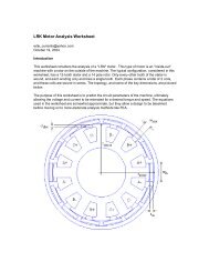
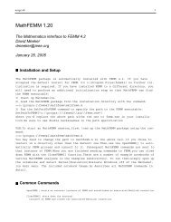
This example, as shown below in Figure 1, the outer square has a 4 cm size and the inner square<br />
has a 2 cm size. The geometry extends for 100 cm in the “into-the-page” direction. The dielectric<br />
between the plates is air. We seek to build the problem, analyze it, and determine the capacitance.<br />
1 This document is based on the "Introduction to FEA with FEMM" tutorial by Ian Stokes-Rees, TSS (UK) Ltd.<br />
Many thanks to Kostadin Brandisky of the Technical University of Sofia for developing the example problems used<br />
in this tutorial.
2<br />
1.5<br />
1<br />
0.5<br />
0<br />
-0.5<br />
-1<br />
-1.5<br />
-2<br />
-2 0 2<br />
y<br />
Figure 1: Square Cross-Section Capacitor<br />
Because of the symmetry, only one quarter of the device need be modeled. The finished model<br />
will look as pictured below in Figure 2 when ready for analysis.<br />
Figure 2: Completed example in the electrostatics preprocessor.<br />
x
The steps required to create this model are as follows:<br />
2.1 Create model<br />
Start FEMM by select the "femm 4.0" entry placed in the "femm 4.0" section of your start menu.<br />
After the program starts, "File|New" from the main menu. Select "<strong>Electrostatics</strong> Problem" in the<br />
"Create a new problem" dialog that appears. After you hit "OK", a blank electrostatics problem<br />
will appear.<br />
Select “nodes” from the tool bar (this is the farthest button on the left with a small black box: )<br />
and place 6 nodes for the corner of a box (at, for example, (0,1), (1,1), (1,0) ,(2,0),(2,2) and (0,2)).<br />
One can place nodes either by moving the mouse pointer to the desired location and pressing the<br />
left mouse button, or by pressing the key and manually entering the point coordinates via<br />
a popup dialog.<br />
Select “lines” from the tool bar (second button from the left with a blue line: ). To select a<br />
node to be the endpoint of a line, click near each desired endpoint with the left mouse button.<br />
Select connect the points as pictured in Figure 2 using this mouse endpoint selection approach.<br />
2.2 Add materials to the model<br />
Select “Properties|Materials” off of the main menu. In the dialog that appears, click the “Add<br />
Material” button. A dialog will pop up with edit boxes for the various material properties.<br />
Change the name of the property from “New Material” to “air.” By default the permittivity of a<br />
new material is 1, which is what we require for air. Press the “OK” button to complete the<br />
creation of the material.<br />
2.3 Define materials for each region<br />
Now click on “Block Labels” (the tool bar button with green circles ), and place a block label<br />
in the middle of the solution domain, between the inner and outer squares. Like node points, block<br />
labels can be placed either by a click on the left mouse button, or via the dialog.<br />
Right click on the block label node for the outer box so that the node turns red, denoting that it is<br />
selected. Press space to “open” the selected block label. A dialog will pop up containing the<br />
properties assigned to the selected label. Set the “Block type” to “Air”. Uncheck the “Let<br />
Triangle choose Mesh Size” checkbox and enter “0.025” for the “Mesh size”. The mesh size<br />
parameter defines a constraint on the largest possible elements size allowed in the associated<br />
section. The mesh generator attempts to fill the region with nearly equilateral triangles in which<br />
the sides are approximately the same length as the specified “Mesh size” parameter. When the<br />
“Let Triangle choose Mesh Size” box is checked, the mesh generator is free to pick its own<br />
element size, usually resulting in a somewhat coarse mesh.
2.4 Define Conductor voltages<br />
Select “Properties|Conductors” from the menu bar, then click on the “Add Property” button.<br />
Replace the name “New Conductory” with “zero”. Select the “Prescribed Voltage” radio button.<br />
Enter a 0 as the value in the associated edit box and Hit “OK”. You have just defined a conductor<br />
that is fixed a voltage of 0V, but you have yet to assign this condition to a particular part of the<br />
model.<br />
Repeat the above process but instead name the new boundary condition “one” and apply enter a<br />
prescribed voltage value of 1.<br />
Select “lines” from the toolbar then right click on the each of the two segments belonging to the<br />
inner conductor. When a segment turns red, you have selected it. Now press space bar and the<br />
“Segment Properties” window will appear. From the “In Conductor” drop box change the<br />
selection from “” to “one”. Repeat this process for the outer conductor, but set the<br />
conductor type to “zero”.<br />
(N.B. for arcs or segments with a prescribed voltage, it is permissible to define a “Fixed Voltage”<br />
boundary condition in lieu of defining a fixed-voltage conductor property. The advantage of<br />
defining the boundaries as conductors, rather than simple boundary conditions, is that charge on<br />
the conductor is calculated automatically in the solver.)<br />
2.5 Set Problem Characteristics<br />
Select “Problem” from the menu bar. In the dialog that appears, make sure the problem type is<br />
“planar”. Set the length units to “Centimeters” and set the “depth” parameter to 100. The default<br />
solver precision of 10 -8 (i.e. solution determined to single precision accuracy) generally need not<br />
be modified. If desired, a descriptive commend can be added in the “Comment” edit box.<br />
2.6 Generate Mesh and Run FEA<br />
Now save the file and click on the toolbar button with yellow mesh: . This action generates a<br />
triangular mesh for your problem. If the mesh spacing seems to fine or too coarse you can select<br />
block labels or line segments and adjust the mesh size defined in the properties of each object.<br />
When you are satisfied with the mesh, click on the “turn the crank” button to run the FEA<br />
algorithm over your model.<br />
Processing status information will be displayed in a dialog box while the solver runs. If the<br />
progress bars do not seem to be moving then you should probably cancel the calculation. This can<br />
occur if insufficient boundary conditions have been specified. For this particular problem, the<br />
calculations should be completed in less than a second (although the solution time is highly<br />
dependent on the speed of the machine running the analysis). There is no confirmation for when<br />
the calculations are completed, the status window just disappears when the processing is finished.<br />
2.7 Display Results
Click on the glasses icon to open the solution in a postprocessor window. The solution will<br />
then be displayed, as pictured in Figure 3. By default, a color density plot of voltage is displayed<br />
when the postprocessor starts. If desired, the default behaviors can be changed via the<br />
Edit|Preferences selection on the main menu of both the preprocessor and postprocessor.<br />
The charge on each conductor can then be determined by selecting View|Conductor Props off of<br />
the postprocessor main menu. A dialog will then appear that displays the voltage and total charge<br />
for each defined conductor. For the “one” conductor, the reported charge is 2.26835e-011<br />
Coulombs. One can use the fact that charge is equal to the product of capacitance and voltage<br />
difference to determine the capacitance of the system. Since only ¼ of the total geometry is<br />
modeled, the total charge is 9.0734e-011 Coulombs. In this case the voltage drop is 1 V,<br />
implying that the total capacitance is 90.734 pF.<br />
Figure 3: Solution to the example rendered in the electrostatics postprocessor.<br />
From this basic introduction you should have gained the following principles:<br />
• How to create your model space using nodes and lines.<br />
• How to add material types to your model and how to assign them to regions.<br />
• How to specify the finite element mesh size.<br />
• How to define conductor properties for your model.<br />
• How to apply conductor properties to line segments in the model.<br />
• How to run the mesh generator and solver.
• How to run the postprocessor and display the resulting charge and voltage on each<br />
conductor.<br />
A completed version of this example problem is available as bdemo1.fee<br />
3. Additional Concepts: Capacitance Between Two Spheres<br />
You will now create a model of a capacitor consisting of two conducting spheres at equal and<br />
opposite voltages sitting in an unbounded region. This is an example of an axisymmetric system,<br />
and a special “open” boundary condition will be used to mimic the behavior of an unbounded<br />
domain.<br />
70.00<br />
25.00 R<br />
25.00 R<br />
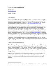
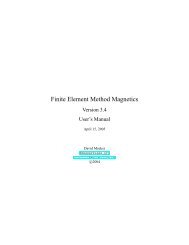
Figure 4: Two conducting spheres.<br />
The arrangement of spheres is pictured in Figure 4. Two spheres, each 25 meters in diameter, are<br />
separated by a center-to-center distance of 70 meters. The top sphere is at a potential of 100<br />
Volts, and the bottom sphere is at a potential of -100 Volts.<br />
Due to symmetry considerations, only one sphere need be model. The line of symmetry between<br />
the two spheres is then fixed at 0 Volts to account for the effects of the second sphere.<br />
We will use the “Asymptotic Boundary Condition” method (as described in the Appendix to the<br />
FEMM manual) to mimic an unbounded geometry. To apply this boundary condition, the finite<br />
element problem domain must be spherical (or circular for a 2D planar problem). When finished<br />
the modeled domain will look as pictured in Figure 5.
Figure 5: Example geometry shown in the electrostatics preprocessor.<br />
First set the “Problem” properties to axisymmetric, and units of meters. Since the problem is<br />
axisymmetric, no Depth entry is required, and that edit box is grayed-out. In this case, the vertical<br />
axis is the axis of rotation for the problem. The r axis runs horizontally, and the z axis runs<br />
vertically.<br />
Change the “Grid Size” to 10, meaning each dot represents a 10 meter increment, and select<br />
snap-to-grid by pushing in the toolbar icon. Snap-to-grid allows points and block labels to be<br />
placed exactly on grid points using clicks of the left mouse button.<br />
Select View|Keyboard. This selection pops up a dialog allowing you to enter the size of the view<br />
via the keyboard. In this dialog, specify the lower-left corner of the screen to be at 0,0 and the<br />
upper right corner to be at (150,150). A view is then picked that contains the prescribed area as is<br />
best possible.<br />
Place a nodes at (r,z) = (0,0), (0,10), and (0,60), (0,150) and (150,0) (refer to the left side of the<br />
status bar at the bottom of the screen for a read-out of the current mouse pointer position).<br />
Connect lines from (0,0) to (0,10)and from (0,60) to (0,150). These lines are located along the<br />
axis of rotation for this axisymmetric problem. Also draw a line from (0,0) to (150,0), along the<br />
axis of symmetry between the two spheres.
Select the arc toolbar button . Select the (0,10) point (bottom point), then select the (0,60)<br />
point (top point). When the dialog box comes up, enter “180” for “Arc Angle” and “1” for “Max.<br />
Segment, Degrees”. The circles are ultimately represented as many-sided polygons, and the<br />
“Max. Segment” parameter prescribes the biggest arc that is allowed to be spanned by any one<br />
side of the polygon. A 1 degree constraint represents a fairly fine discretization—the default is 10<br />
degrees. In the postprocessor, all arcs are drawn counter clockwise, so this will draw the halfcircle<br />
defining the outside of one of the conducting spheres.<br />
Now select the (150,0) point followed by the (0,150) point, and enter “90” for “Arc Angle” and<br />
“1” for “Max. Segment”. This arc will be the exterior boundary of the finite element solution<br />
domain.<br />
Deselect “snap-to-grid,” switch to “block label” mode (by pressing ), and place a block label<br />
(green node) inside the closed region between the outer surface of the conducting sphere and the<br />
arc representing the exterior boundary<br />
Add “Air” to the model’s materials using the “Properties|Materials” main menu selection, as<br />
described in Example 1.<br />
Select “Properties|Conductors” from the menu and create a conductor named “+100V” with a<br />
prescribed voltage of 100 Volts (procedure as described above in Example 1).<br />
Create a fixed voltage boundary for the line of symmetry. Do this by selecting<br />
“Properties|Boundary” off of the main menu. Click the “Add Property” button and make a<br />
property named “zero” that has a prescribed voltage of 0.<br />
Add a second block label that will be used as the condition on the exterior boundary. Rename<br />
your new boundary “open_bc” and change the “BC Type” to “Mixed”. Given that the system<br />
under analysis is close to the center of an arc (usually either a full or half circle), “c0 coefficient”<br />
can be set to ( 2 o / r ε ) where r is the radius of the arc in meters. In this case, you can let the<br />
program do the most of the appropriate calculations by entering the string:<br />
2*eo/150<br />
into the edit box for the c0 coefficient (the c1 coefficient should be zero). The quantity eo has<br />
been predefined to contain the permeability of free space in SI units, and we are exploting the fact<br />
that the contents of every edit in FEMM box gets parsed by the Lua scripting language, enabling<br />
formulas to be entered in any edit box in which a numerical value is required.<br />
Select the quarter-circle arc representing the exterior boundary by right clicking on or near it (the<br />
“Arc” toolbar button must also be depressed). Press space and assign the boundary condition to be<br />
“open_bc”.
Select the half-circle representing the surface of one of the conducting spheres. Press space and<br />
assign “+100V” as the conductor for property for this surface.<br />
Switching to Segment mode, assign the “zero” boundary condition to the line of symmetry at z=0.<br />
In Block Mode, select the block label inside the domain by right clicking with the mouse near the<br />
green node. Change the “Block type” to Air and the “Mesh size” to 1.<br />
Now generate the mesh, perform the calculation, and open the solution in a postprocessor window<br />
to display the resulting voltages, all in the same way as described in Example 1. The resulting<br />
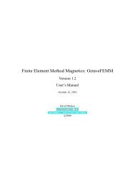
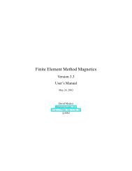
solution should look as pictured in Figure 6.<br />
Figure 6: Solution to the example as rendered in the electrostatics postprocessor<br />
Note that the vertical side of the semi-circle boundary (along the radial axis) does not have any<br />
boundary condition assigned—an “insulated” boundary condition is defined to the axis of rotation<br />
in axisymmetric problems by default. Also note how the equipotential lines radiate through the<br />
outer arc boundary as if heading to infinity. This is due to the use of an impedance boundary<br />
condition on the outer boundary, which closely mimics the behavior of the spheres in unbounded<br />
free space.<br />
By selecting View|Conductor Props from the main menu (or by pushing the button), one<br />
obtains a charge of 4.4769e-007 Coulombs on the sphere.
Force on the sphere can also be evaluated. Switch to the block postprocessor mode by press the<br />
block button. To select the surface of the conducting sphere for force integration, click on the<br />
sphere’s surface with the right mouse button. When a conductor is selected, it is rendered in red.<br />
(In other problems in which force on a volume, rather than a surface, is desired, the volume can<br />
be selected with a left mouse button click). Then, press the integral toolbar button and select<br />
“Force via weighted stress tensor” from the drop list in the dialog that appears. This is probably<br />
the most accurate way to determine forces in FEMM on objects that are completely surrounded by<br />
air. The resulting force on the top sphere is -4.730649e-007 N from the FEMM model.<br />
For comparison purposes, it is interesting to re-run the analysis with the “zero” boundary<br />
condition applied to the exterior boundary. With a “Zero” outer boundary, the ground is at a finite<br />
distance, rather than being located at infinity. In this case, the charge is 4.58617e-007<br />
Coulombs—the presence of the artificial boundary slightly elevates the capacitance of the system.<br />
From this second example, you should have gained the following additional principles:<br />
• How to define circles and arcs in the proprocessor.<br />
• How to create an “open” boundary condition for the analysis of an unbounded problem.<br />
• How to run compute force on a conductor.<br />
A completed version of this example problem is available as bdemo2.fee<br />
4. Conclusions<br />
The finite element solutions to some fairly simple problems in electrostatics have been presented<br />
in a step-by-step fashion. Hopefully, these examples will allow you to apply the program to<br />
practical problems with more complicated geometries.