Magnetics Tutorial - Finite Element Method Magnetics

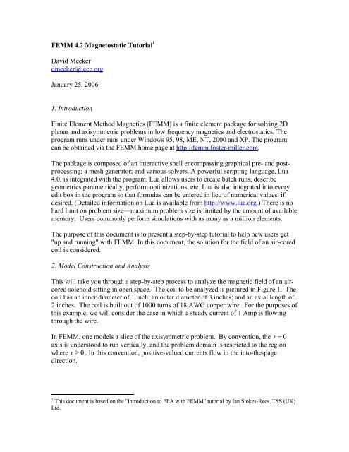
FEMM 4.2 Magnetostatic Tutorial 1
David Meeker
dmeeker@ieee.org
January 25, 2006
1. Introduction
Finite Element Method Magnetics (FEMM) is a finite element package for solving 2D
planar and axisymmetric problems in low frequency magnetics and electrostatics. The
program runs under runs under Windows 95, 98, ME, NT, 2000 and XP. The program
can be obtained via the FEMM home page at http://femm.foster-miller.com.
The package is composed of an interactive shell encompassing graphical pre- and postprocessing;
a mesh generator; and various solvers. A powerful scripting language, Lua
4.0, is integrated with the program. Lua allows users to create batch runs, describe
geometries parametrically, perform optimizations, etc. Lua is also integrated into every
edit box in the program so that formulas can be entered in lieu of numerical values, if
desired. (Detailed information on Lua is available from http://www.lua.org.) There is no
hard limit on problem size—maximum problem size is limited by the amount of available
memory. Users commonly perform simulations with as many as a million elements.
The purpose of this document is to present a step-by-step tutorial to help new users get
"up and running" with FEMM. In this document, the solution for the field of an air-cored
coil is considered.
2. Model Construction and Analysis
This will take you through a step-by-step process to analyze the magnetic field of an aircored
solenoid sitting in open space. The coil to be analyzed is pictured in Figure 1. The
coil has an inner diameter of 1 inch; an outer diameter of 3 inches; and an axial length of
2 inches. The coil is built out of 1000 turns of 18 AWG copper wire. For the purposes of
this example, we will consider the case in which a steady current of 1 Amp is flowing
through the wire.
In FEMM, one models a slice of the axisymmetric problem. By convention, the r = 0
axis is understood to run vertically, and the problem domain is restricted to the region
where r ≥ 0 . In this convention, positive-valued currents flow in the into-the-page
direction.
1 This document is based on the "Introduction to FEA with FEMM" tutorial by Ian Stokes-Rees, TSS (UK)
Ltd.

2.1 Create a New Model
Figure 1: Air-cored coil to be analyzed in first example.
Run the FEMM application by selecting femm 4.0 from the femm 4.0 section of the Start
Menu. The default preferences will bring up a blank window with a minimal menu bar.
Select New from the main menu. A dialog will pop up with a drop list allowing you to
select the type of new document to be created. Select the Magnetics Problem entry and hit
the OK button. A new blank magnetics problem will be created, and a number of new
toolbar buttons will appear.
2.2 Set Problem Definition
The first task is to tell the program what sort of problem is to be solved. To do this,
select Problem from the main menu. The Problem Definition dialog will appear. Set
Problem Type to Axisymmetric. Make sure that Length Units is set to Inches and that the
Frequency is set to 0. When the proper values have been entered, hit the OK button.
2.3 Draw Boundaries
The first task is to draw boundaries for the solution region. Fundamentally, finite
element solvers mesh and find a solution over a finite region of space that contains the
objects of interest. In this case, we will choose our solution region to be a sphere with a
radius of 4 inches.
First, we can adjust the view so that it will contain the entire solution region. Select
View|Keyboard off of the main menu to bring up a dialog that allows you to specify the
extents of the visible screen. In this dialog, specify Bottom to be -4, Left to be 0, Right to
be 4, and Top to be 4 and hit the OK button. The screen will then be rescaled to the
smallest rectangle that contains the specified region.

Next, node points need to be defined that bound the sphere. To draw these node points,
select the Operate on nodes button from the from the tool bar (this is the farthest button
on the left with a small black box: ) . Place nodes at the top and bottom of the sphere,
at (0,4) and (0-4), and at the origin (0,0). One can place nodes either by moving the
mouse pointer to the desired location and pressing the left mouse button, or by pressing
the key and manually entering the point coordinates via a popup dialog.
Select the Operate on segments toolbar button (second button from the left with a blue
line: ). To select a node to be the endpoint of a line, click near the desired endpoint
with the left mouse button. Draw a line down the axis of symmetry by selecting the point
at (0,-4) and then the point at (0,4). A line will appear linking the nodes as soon as the
second point is selected.
Select the Operate on arc segments toolbar button (third button from the left with a blue
arc: ). Draw an arc down the axis of symmetry by selecting the point at (0,-4) and
then the point at (0,4). A dialog will appear asking you for some attributes of the arc. In
FEMM, arc are approximated by a series of small, straight lines. The Max. segement
specifies the coarseness with which the arc is divided into sections. Enter 2.5 into this
edit box to get a fairly fine representation of the arc. Put 180 in the Arc Angle edit box to
denote that a half circle is being drawn.
2.4 Draw Coil
Now, the coil itself can be drawn. Switch back to Nodes mode by pressing the the
Operate on nodes toolbar button. Place nodes at (0.5,-1), (1.5,-1), (1.5,1) and (0.5,1)
defining the extents of the coil. Select the Operate on segments toolbar button so that
lines can be drawn connecting the points. By selecting the nodes defining the coil in
sequence, one obtains lines between each of the nodes and result in a large connected
box.
2.5 Place Block Labels
Now click on the Operate on Block Labels toolbar button denoted by concentric green
circles . Place a block label in the coil region, and place one in the air outside the coil
region. Like node points, block labels can be placed either by a click on the left mouse
button, or via the dialog. The program uses block labels to associate materials
and other properties with various regions in the problem geometry. Next, we will defined
some material properties, and then we will go back and associate them with particular
block labels.
NOTE: If snap-to-grid is enabled then it may be sometimes be difficult to place the block label in the empty
space. If this is the case, disable snap-to-grid by de-selecting the tool bar button with the point and arrow.
2.6 Add materials to the model

Select Properties|Materials Library off of the main menu. The drag-and-drop Air from
Library Materials to Model Materials to add it to the current model. Go into the Copper
AWG Sizes folder and drag 18 AWG into Model Materials. Click on OK.
2.7 Add a "Circuit Property" for the coil
Select Properties|Circuits off of the main menu. On the dialog that appears, push the Add
Property button to create a new circuit property. Name circuit by replacing the new
circuit name with Coil. Specify that the circuit property is to be applied to a wound region
by selecting the Series radio button. Enter 1 as the Circuit Current. The j edit box denotes
the imaginary component of the current, which is used in time harmonic problems to
denote the phase of the current. In this case, the problem is magnetostatic, so the
imaginary component is ignored—just put zero in the j edit box. Click on OK for both the
Circuit Property and Property Definition dialogs.
2.8 Associate properties with block labels.
Right click on the block label node in the air region outside the coil. The block label will
turn red, denoting that it is selected. Press space to “open” the selected block label
(Instead of pressing the space bar, one can use the Open up Properties Dialog toolbar
button ) . A dialog will pop up containing the properties assigned to the selected label.
Set the Block type to Air. Uncheck the Let Triangle choose Mesh Size checkbox and enter
0.1 for the Mesh size. The mesh size parameter defines a constraint on the largest possible
elements size allowed in the associated section. The mesher attempts to fill the region
with nearly equilateral triangles in which the sides are approximately the same length as
the specified Mesh size parameter. When the “Let Triangle choose Mesh Size” box is
checked, the mesher is free to pick its own element size, usually resulting in a somewhat
coarse mesh. Click on OK. The block label will then be labeled as Air, and a circle will
appear about the block label indicating the approximate mesh size in the associated
region.
Repeat the same for the block label node inside the coil region, changing the mesh size to
0.1. However, set this Block type to Copper. We want to assign currents to flow in this
region, so select the Coil circuit from the In Circuit drop list. The Number of turns edit box
will become activated if a series-type circuit is selected for the region (e.g the Coil
property that was previously defined). Enter 1000 as the number of turns for this region,
denoting that the region if filled with 1000 turns wrapped in a counter-clockwise
direction (i.e. positive turns in the right-hand-screw rule sense). Click on OK.
NOTE: If we wanted to denote that the turns are wrapped in a counter-clockwise direction instead, we
could have specified the number of turns to be –1000.
2.9 Create Boundary Conditions

Select Properties|Boundary from the menu bar, then click on the Add Property button.
Replace the name New Boundary with ABC and change the BC Type to Mixed. The ABC
name is meant to denote that we are creating an "asymptotic boundary condition" that
approximates the impedance of an unbounded, open space. In this way, we can model
the field produced by the coil in an unbounded space while still only modeling a finite
region of that space. When the Mixed boundary condition type is selected the c0
coefficient and c1 coefficient boxes will become enabled. These entries are meant to
represent coefficients in a boundary condition of the form:
1 ∂ A
+ cA o + c1=
0
µµ ∂n
r o
where A is magnetic vector potential, µr is the relative magnetic permeability of the
region adjacent to the boundary, µo is the permeability of free space, and n represents the
direction normal to the boundary. For our asymptotic boundary condition, we need to
specify:
1
co
=
µ rµ oR
c = 0
1
where R is the outer radius of a spherical problem domain. To enter these values into the
dialog box, enter 0 as the c1 coefficient and 1/(uo*4*inch) as the c0 coefficient. The Lua
scripting language processes the contents of each edit box automatically when the dialog
is closed, substituting the numerical value of the permeability of free space for uo and
0.0254 for inch and evaluating the result.
To assign this boundary condition, switch to Operate on arc segments mode. Select the
arc defining the outer boundary by clicking on the arc with the left mouse button and
push the space bar to open the arc's properties for editing. Select ABC from the Boundary
cond. drop list and click on OK. You have now defined enough boundary conditions to
solve the problem, since a zero potential is automatically applied along the r = 0 line for
axisymmetric problems.
You have now completed modeling the coil. The finished pre-processor geometry should
look as pictured in Figure 2.

Figure 2: Completed coil model, ready to be analyzed.
2.10 Generate Mesh and Run FEA
Now save the file and click on the toolbar button with yellow mesh: . This action
generates a triangular mesh for your problem. If the mesh spacing seems to fine or too
coarse you can select block labels or line segments and adjust the mesh size defined in
the properties of each object. Once the mesh has been generated, click on the “turn the
crank” button to analyze your model.
Processing status information will be displayed. If the progress bars do not seem to be
moving then you should probably cancel the calculation. This can occur if insufficient
boundary conditions have been specified. For this particular problem, the calculations
should be completed within a second. There is no confirmation for when the calculations
are complete, the status window just disappears when the processing is finished.
3. Analysis Results

Click on the glasses icon to view the analysis results. A post-processor window will
appear. The post-processor window will allow you to extract many different sorts of
information from the solution.
3.1 Point values
Just like the pre-processor, the post-processor window has a set of different editing
modes: Point, Contour, and Area. The choice of mode is specified by the mode toolbar
buttons, i.e. where the first button corresponds to Point mode, the second to
Contour mode, and the third to Area mode. By default, when the program is first
installed, the post-processor starts out in Point mode. By clicking on any point with the
left mouse button, the various field properties associated with that point are displayed in
the floating FEMM Output window. Similar to drawing points in the pre-processor, the
location of a point can be precisely specified by pressing the button and entering
the coordinates of the desired point in the dialog that pops up. For example, if the point
(0,0) is specified in the pop-up dialog, the resulting properties displayed in the output
window are as pictured in Figure 3.
3.2 Coil terminal properties
Figure 3: Display of field values at the point (0,0).
With FEMM, it is straightforward to determine the inductance and resistance of the coil
as seen from the coil's terminals. Press the button to display the resulting attributes of
each Circuit Property that has been defined. For the Coil property defined in this example,
the resulting dialog is pictured in Figure 4.

Figure 4: Circuit Property results dialog.
Since the problem is linear and there is only one current, the Flux/Current result can be
unambiguously interpreted as the coil's inductance (i.e. 22.9 mH). The resistance of the
coil is the Voltage/Current result (i.e. 3.34 Ω).
3.3 Plotting field values along a contour
FEMM can also plot values of the field along a user-defined contour. Here, we will plot
the flux density along the centerline of the coil. Switch to Contour mode by pressing the
Contour Mode toolbar button. You can now define a contour along which flux will be
plotted. There are three ways to add points to a contour:
1. Left Mouse Button Click adds the nearest input node to the contour;
2. Right Mouse Button Click adds the current mouse pointer position to the contour;
3. Key displays a point entry dialog that allows you to enter in the
coordinates of a point to be added to the contour.
Here, method 1 can be used. Click near the node points at (0,4), (0,0), and (0,-4) with the
left mouse button, adding the points in the above order. Then, press the Plot toolbar
button . Hit OK in the X-Y Plot of Field Values pop-up dialog—the default selection
is magnitude of flux density. If desired, different types of plot can be selected from the
drop list on this dialog.
NOTE: It is often the case in the solution to magnetic problems that the field values are discontinuous
across a boundary. In this case, FEMM determines which side of the boundary will be plotted based on the
order in which points are added. For example, if points are added around a closed contour in a counterclockwise
order, the plotted points will lie just to the inside of the contour. If the points are added in a
clockwise order, the plotted points will lie just to the outside of the contour. The implication to our
example problem is that the contour along the r=0 should be defined in order of decreasing z (i.e. counterclockwise
so that the plotted points will lie inside the solution domain instead of outside it, where the field
values are not defined).

3.4 Plotting Flux Density
By default, when the program is first installed, only a black-and-white graph of flux lines
is displayed. Flux density can be plotted as a color density plot, if you so desire. To
make a color density plot of flux, click on the purple shaded toolbar button to
generate a color flux density plot. When the dialog box comes up, select the Flux density
plot radio button and accept the other default values. Click on OK. The resulting solution
view will look similar to that pictured in Figure 4.
4. Conclusions
Figure 4: Color flux density plot of solution.
You have now completed your first model of a magnetic problem with FEMM. From this
basic introduction, you have been exposed to the following concepts:

• How to draw a model using nodes, segments, arc, and block labels;
• How to add material to your model and how to assign them to regions;
• How to specify the finite element mesh size;
• How to define boundary for your model;
• How to define and apply boundary conditions;
• How to analyze a problem;
• How to inspect local field values;
• How to plot field values along a line;
• How to compute inductance and resistance;
• How to display color flux density plots.
Hopefully, this tutorial has presented you with enough of the basics of FEMM so that you
can explore more complicated problems without getting sidetracked by the mechanics of
how a problem is drawn and analyzed.