Spectral Estimation Using a MUSIC Algorithm - Altera

More documents

Recommendations

Info

Spectral Estimation Using a MUSIC Algorithm The hardware-software co-simulation in the ModelSim ® tool helped me to resolve the problem, and to estimate the time taken by the processor to acknowledge the interrupt. The program developed for the back substitution is not fixed for four antenna elements, but it is a general program, applicable to any number of antenna elements. The Avalon bus is a simple bus architecture designed for connecting on-chip processors and peripherals together into a system-on-a-programmable-chip (SOPC) solution. See Figure 14. It is an interface that specifies the port connections between master and slave components. Basic Avalon bus transactions transfer a single byte, half word, or word between a master and slave peripheral. After the completion of a transfer, the bus is available on the next clock cycle for any another transaction. Figure 14. Avalon Bus Avalon Bus Nios II Processor C_r C_i Data & Program Memory R_r R_i U_r U_i Mixed Mode EVD_Decomposer Some key features of the Avalon bus are: ■ ■ ■ ■ ■ ■ Memory and peripherals may be mapped anywhere within the 32- bit address space. All Avalon signals are synchronized to the Avalon bus clock, which simplifies the timing behavior of the Avalon bus and facilitates integration with high-speed peripherals. Separate, dedicated address and data paths provide the easy interface to on chip user logic. Peripherals do not need to decode data and address bus cycles. The Avalon bus automatically generates chip select signals for all peripherals, greatly simplifying the design of Avalon peripherals. Multiple master peripherals can reside on the Avalon bus. The Avalon bus generates the required arbitration logic. The Avalon bus also handles the details of transferring data between peripherals with mismatched data widths. Device Utilization Summary Family Stratix Device EP1S10F780C6ES Total logic elements 8,236 / 10,570 ( 77 % ) Total pins 34 / 427 ( 31 % ) Total memory bits 61,856 / 920,448 ( 6 % ) DSP block 9-bit elements 8 / 48 ( 16 % ) Total phase-locked loops (PLLs) 1 / 6 ( 16 % ) Total DLLs 0 / 2 ( 0 % ) 85
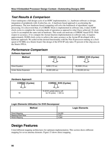
Nios II Embedded Processor Design Contest—Outstanding Designs 2005 Test Results & Comparison I have undergone a full design cycle of an SOPC implementation, i.e., hardware-software co-design, integration of peripherals with Avalon bus, etc. A hardware-based approach is accelerating the performance. The new hardware-based computing will solve the bottleneck of algorithmic signal processing. It is discovered that, if a CORDIC block is implemented in software only, it takes 8,600 clock cycles to complete the vectoring mode of operation as opposed to what I have achieved: 16 clock cycles to accomplish the same task in hardware. This result can motivate a CORDIC-based EVD. With respect to accuracy, if we compare the Arctan function implementation in software only, it requires approximately 20,000 clock cycles to achieve the same accuracy as the Arctan IP developed with a hardware approach. We achieved the desired functionality with the Nios II processor running at a clock speed of 50 MHz on a Stratix board. Our design of the EVD IP only takes 55 percent of the chip area on the Stratix FPGA. Performance Comparison Software Approach Method CORDIC (Cycles) CORDIC EVD (Cycles) Direct Equation 8,600 (172 us) 90,3000 (18 us) Arctan Series Expansion 20,000 (400 us) 2,100,000 (42 ms) Hardware Approach CORDIC (Cycles) CORDIC EVD (Cycles) 16 16 (EVD update latency will be 16 cycles) = 320 ns Logic Elements Utilization for EVD Decomposer Method Logic Elements Direct Mapping 34,055 Mapping Each Row 7,811 Mixed Mapping 4,946 Design Features I tried different mapping architectures for optimum implementation. This section shows different mapping for seven antenna elements. Figure 15 shows direct mapping. 86
Page 1 and 2: Nios II Embedded Processor Design C
Page 11: Nios II Embedded Processor Design C

Spectral Estimation Using a MUSIC Algorithm - Altera

Create successful ePaper yourself

Delete template?

Save as template?