Demystifying Auto-Zero Amplifiers—Part 1 - Analog Devices

A forum for the exchange of circuits, systems, and software for real-world signal processing
SSB UPCONVERSION OF QUADRATURE DDS SIGNALS TO THE 800-TO-2500-MHz BAND (page 46)
Fundamentals of DSP-Based Control for AC Machines (page 3)
Transducer/Sensor Excitation and Measurement Techniques (page 33)
Complete contents on page 1
Volume 34, 2000
a

About Analog Dialogue
Analog Dialogue is the free technical magazine of Analog Devices, Inc., published continuously
for thirty-four years, starting in 1967. It discusses products, applications, technology, and
techniques for analog, digital, and mixed-signal processing.
Volume 34, the current issue, incorporates all articles published during 2000 in the
World Wide Web editions www.analog.com/analogdialogue. All recent issues,
starting with Volume 29, Number 2 (1995) have been archived on that website and
can be accessed freely.
Analog Dialogue’s objectives have always been to inform engineers, scientists, and
electronic technicians about new ADI products and technologies, and to help them
understand and competently apply our products.
The frequent Web editions have at least three further objectives:
• Provide timely digests that alert readers to upcoming and newly available products.
• Provide a set of links to important and rapidly proliferating sources of information
and activity fermenting within the ADI website [www.analog.com].
• Listen to reader suggestions and help find sources of aid to answer their questions.
Thus, Analog Dialogue is more than a magazine: its links and tendrils to all
parts of our website (and some outside sites) make its bookmark a favorite
“high-pass-filtered” point of entry to the analog.com site—the virtual world of
Analog Devices.
Our hope is that readers will think of ADI publications as “Great Stuff” and the
Analog Dialogue bookmark on their Web browser as a favorite alternative path to
answer the question, “What’s new in technology at ADI?”
Welcome! Read and enjoy!
We encourage your feedback*!
Dan Sheingold
dan.sheingold@analog.com
Editor, Analog Dialogue
*We’ve included a brief questionnaire in this issue (page 55); we’d be most grateful if you’d answer the
questions and fax it back to us at 781-329-1241.
© 2000 and 2001 Analog Devices, Inc., all rights reserved

IN THIS ISSUE
Analog Dialogue Volume 34, 2000
Page
Editor’s Notes: New Fellow, Authors . . . . . . . . . . . . . . . . . . . . . . . . . . . . . . . . . . . . . . . . . . . . . . 2
Fundamentals of DSP-Based Control for AC Machines . . . . . . . . . . . . . . . . . . . . . . . . . . . . . . . . . . 3
Embedded Modems Enable Appliances to Communicate with Distant Hosts via the Internet . . . . . . . . . . 7
Adaptively Canceling Server Fan Noise . . . . . . . . . . . . . . . . . . . . . . . . . . . . . . . . . . . . . . . . . . . . 10
Fan-Speed Control Techniques in PCs . . . . . . . . . . . . . . . . . . . . . . . . . . . . . . . . . . . . . . . . . . . . . . 16
Finding the Needle in a Haystack—Measuring Small Voltages Amid Large Common Mode . . . . . . . . . 21
Demystifying Auto-Zero Amplifiers—Part 1 . . . . . . . . . . . . . . . . . . . . . . . . . . . . . . . . . . . . . . . . . . 25
Demystifying Auto-Zero Amplifiers—Part 2 . . . . . . . . . . . . . . . . . . . . . . . . . . . . . . . . . . . . . . . . . . 28
Curing Comparator Instability with Hysteresis . . . . . . . . . . . . . . . . . . . . . . . . . . . . . . . . . . . . . . . . 30
Transducer/Sensor Excitation and Measurement Techniques . . . . . . . . . . . . . . . . . . . . . . . . . . . . . . . 33
Advances in Video Encoders . . . . . . . . . . . . . . . . . . . . . . . . . . . . . . . . . . . . . . . . . . . . . . . . . . . . 38
Selecting an Analog Front-End for Imaging Applications . . . . . . . . . . . . . . . . . . . . . . . . . . . . . . . . . 40
True RMS-to-DC Measurements, from Low Frequencies to 2.5 GHz . . . . . . . . . . . . . . . . . . . . . . . . 45
Single-Sideband Upconversion of Quadrature DDS Signals to the 800-to-2500-MHz Band . . . . . . . . 46
VDSL Technology Issues—An Overview . . . . . . . . . . . . . . . . . . . . . . . . . . . . . . . . . . . . . . . . . . . . 50
Authors (continued from page 2) . . . . . . . . . . . . . . . . . . . . . . . . . . . . . . . . . . . . . . . . . . . . . . . . 53
Feedback Questionnaire . . . . . . . . . . . . . . . . . . . . . . . . . . . . . . . . . . . . . . . . . . . . . . . . . . . . . . . 55
Cover: The cover illustration was designed and executed by Kristine Chmiel-Lafleur, of Communications Services, Analog Devices, Inc.

Editor’s Notes
We are pleased to note the introduction
of Dr. David Smart as new
Fellow at our 2000 General Technical
Conference. Fellow, at Analog
Devices, represents the highest level
of achievement that a technical
contributor can achieve, on a par
with Vice President. The criteria
for promotion to Fellow are very
demanding. Fellows will have
earned universal respect and recognition from the technical community
for unusual talent and identifiable innovation at the state
of the art. Their creative technical contributions in product or
process technology will have led to commercial success with a
major impact on the company’s net revenues.
Attributes include roles as mentor, consultant, entrepreneur,
organizational bridge, teacher, and ambassador. Fellows must also
be effective leaders and members of teams and in perceiving
customer needs. Dave’s technical abilities, accomplishments, and
personal qualities well qualify him to join Bob Adams (1999),
Woody Beckford (1997), Derek Bowers (1991), Paul Brokaw
(1979), Lew Counts (1983), Barrie Gilbert (1979), Roy Gosser
(1998), Bill Hunt (1998), Jody Lapham (1988), Chris Mangelsdorf
(1998), Fred Mapplebeck (1989), Jack Memishian (1980), Doug
Mercer (1995), Frank Murden (1999), Mohammad Nasser (1993),
Wyn Palmer (1991), Carl Roberts (1992), Paul Ruggerio (1994),
Brad Scharf (1993), Jake Steigerwald (1999), Mike Timko (1982),
Bob Tsang (1988), Mike Tuthill (1988), Jim Wilson (1993), and
Scott Wurcer (1996) as Fellow.
NEW FELLOW
Dave Smart is the chief technologist
behind ADICE, our highly
successful analog and mixed-signal
circuit simulator, which is widely
used by chip designers in Analog
Devices. Dave joined ADI in 1988,
assuming responsibility for ADICE.
He made numerous contributions to
the robustness, accuracy, and features
of the simulator, winning the praise
of Analog Devices’ demanding analog IC designers. To meet the
challenges of designing large mixed-signal chips in the 1990s, Dave
led a small team in the development and deployment of a completely
new version of ADICE with innovative techniques for the
effective simulation of mixed-signal circuits using mixed levels of
modeling abstraction. He is currently working on tools and methods
for the design of RF and high-speed ICs. The work of Dave and
his team has been a key element of the design of nearly every analog
and mixed-signal product developed by Analog Devices in the
past decade.
Dave developed an interest in analog circuits as a teenager growing
up in Skokie, Illinois. Before receiving any formal education in
electronics, he and a friend designed and built an audio mixing
board for their high school auditorium to be used in theatrical
productions. While pursuing his study of circuits as an undergraduate
at the University of Illinois at Urbana-Champaign in the early 1970s,
he became aware of the power of digital computers and imagined
their use to take some of the tedium and guesswork out of circuit
design. Once he met Professor Tim Trick, who was active in the
field of computer-aided design of circuits, Dave’s career direction
was set. After receiving BS and MS degrees from the University of
Illinois, he worked on circuit simulation at GTE Communication
Systems for seven years. He returned to the University of Illinois,
researching parallel algorithms for circuit simulation with Professor
Trick, and he obtained his PhD degree prior to joining ADI in 1988.
THE AUTHORS
Rick Blessington (page 7) rejoined
ADI as a Business Development
Manager in April of 1999, after 15
years in the sales and marketing of
communication products for major
electronics companies. At present,
he is involved in development of
inventive new products under a
contract collaboration between
Sierra Telecom (So. Lake Tahoe) and
Analog Devices. Rick holds BA and MA degrees in Technology
from California State University at Long Beach. In the early years
of his career, Rick taught electronics in Southern California. He
and his family now live in Walpole, MA; his hobbies include sailing
and skiing.
Kevin Buckley (page 40) is a Senior
Applications Engineer in the High-
Speed Converter Division, in
Wilmington, MA, working on analog
front ends for imaging applications.
He joined Analog Devices in 1990 as
a technician for the Microelectronics
Division and received a BSEE in
1997 from Merrimack College,
North Andover, MA. In his spare
time he plays hockey and soccer, coaches his son’s soccer team, and
enjoys chasing his baby daughter around the house.
Paschal Minogue (page 10) is the
Engineering Manager of the Digital
Audio Group in Limerick, Ireland.
He graduated from University
College Dublin, with a B.E.
Electronic Engineering degree (First
Class Honors) and joined the
Design Department at Analog
Devices in Limerick, Ireland, in
1981. Since then, he has worked on
standard converters, noise cancellation, communication products,
and most recently audio-band and voice-band products.
Reza Moghimi (page 28) is an
Applications Engineer for the
Precision Amplifier product line in
Santa Clara, CA. He is responsible
for amplifiers, comparators,
temperature sensors, and the SSM
audio product line. He holds a BS
from San Jose State University and
an MBA from National University
(Sunnyvale, CA). His leisure
interests include playing soccer and
traveling with his family. [more authors on Page 53]
2 ISSN 0161–3626 Analog Dialogue Volume 34 ©Analog Devices, Inc. 2000

Fundamentals of
DSP-Based Control
for AC Machines
by Finbarr Moynihan,
Embedded Control Systems Group
INTRODUCTION
High-performance servomotors are characterized by the need for
smooth rotation down to stall, full control of torque at stall, and
fast accelerations and decelerations. In the past, variable-speed
drives employed predominantly dc motors because of their
excellent controllability. However, modern high-performance
motor drive systems are usually based on three-phase ac motors,
such as the ac induction motor (ACIM) or the permanent-magnet
synchronous motor (PMSM). These machines have supplanted
the dc motor as the machine of choice for demanding servomotor
applications because of their simple robust construction, low
inertia, high output-power-to-weight ratios, and good performance
at high speeds of rotation.
The principles of vector control are now well established for
controlling these ac motors; and most modern high-performance
drives now implement digital closed-loop current control. In such
systems, the achievable closed-loop bandwidths are directly related
to the rate at which the computationally intensive vector-control
algorithms and associated vector rotations can be implemented in
real time. Because of this computational burden, many highperformance
drives now use digital signal processors (DSPs) to
implement the embedded motor- and vector-control schemes. The
inherent computational power of the DSP permits very fast cycle
times and closed-loop current control bandwidths (between 2 and
4 kHz) to be achieved.
The complete current control scheme for these machines also
requires a high-precision pulsewidth modulation (PWM) voltagegeneration
scheme and high-resolution analog-to-digital (A/D)
conversion (ADC) for measurement of the motor currents. In order
to maintain smooth control of torque down to zero speed, rotor
position feedback is essential for modern vector controllers.
Therefore, many systems include rotor-position transducers, such
as resolvers and incremental encoders. We describe here the
fundamental principles behind the implementation of highperformance
controllers (such as the ADMC401) for three-phase
ac motors—combining an integrated DSP controller, with a
powerful DSP core, flexible PWM generation, high-resolution
A/D conversion, and an embedded encoder interface.
VARIABLE SPEED CONTROL OF AC MACHINES
Efficient variable-speed control of three-phase ac machines requires
the generation of a balanced three-phase set of variable voltages
with variable frequency. The variable-frequency supply is typically
produced by conversion from dc using power-semiconductor
devices (typically MOSFETs or IGBTs) as solid-state switches. A
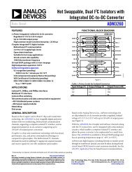
commonly-used converter configuration is shown in Figure 1a. It
is a two-stage circuit, in which the fixed-frequency 50- or 60-Hz
ac supply is first rectified to provide the dc link voltage, V D , stored
in the dc link capacitor. This voltage is then supplied to an inverter
circuit that generates the variable-frequency ac power for the motor.
The power switches in the inverter circuit permit the motor
terminals to be connected to either V D or ground. This mode of
operation gives high efficiency because, ideally, the switch has zero
loss in both the open and closed positions.
By rapid sequential opening and closing of the six switches (Figure
1a), a three-phase ac voltage with an average sinusoidal waveform
can be synthesized at the output terminals. The actual output
voltage waveform is a pulsewidth modulated (PWM) highfrequency
waveform, as shown in Figure 1b. In practical inverter
circuits using solid-state switches, high-speed switching of about
20 kHz is possible, and sophisticated PWM waveforms can be
generated with all voltage harmonic components at very high
frequencies; well above the desired fundamental frequencies—
nominally in the range of 0 Hz to 250 Hz.
The inductive reactance of the motor increases with frequency so
that the higher-order harmonic currents are very small, and nearsinusoidal
currents flow in the stator windings. The fundamental
voltage and output frequency of the inverter, as indicated in Figure
1b, are adjusted by changing the PWM waveform using an
appropriate controller. When controlling the fundamental output
voltage, the PWM process inevitably modifies the harmonic content
of the output voltage waveform. A proper choice of modulation
strategy can minimize these harmonic voltages and their associated
harmonic effects and high-frequency losses in the motor.
THREE-
PHASE
60Hz
MAINS
RECTIFIER
V D
N
INVERTER
A B C
a. Typical configuration of power converter used to drive threephase
ac motors.
FUNDAMENTAL
MOTOR
PHASE
VOLTAGE
V AB
V AN
V BN
DESIRED FREQUENCY
DESIRED
AMPLITUDE
b. Typical PWM waveforms in the generation of a variablevoltage,
variable-frequency supply for the motor.
Figure 1.
M
Analog Dialogue 34-6 (2000) 3

PULSEWIDTH MODULATION (PWM) GENERATION
In typical ac motor-controller design, both hardware and software
considerations are involved in the process of generating the PWM
signals that are ultimately used to turn on or off the power devices
in the three-phase inverter. In typical digital control environments,
the controller generates a regularly timed interrupt at the PWM
switching frequency (nominally 10 kHz to 20 kHz). In the interrupt
service routine, the controller software computes new duty-cycle
values for the PWM signals used to drive each of the three legs of
the inverter. The computed duty cycles depend on both the
measured state of the motor (torque and speed) and the desired
operating state. The duty cycles are adjusted on a cycle-by-cycle
basis in order to make the actual operating state of the motor follow
the desired trajectory.
Once the desired duty cycle values have been computed by the
processor, a dedicated hardware PWM generator is needed to
ensure that the PWM signals are produced over the next PWMand-controller
cycle. The PWM generation unit typically consists
of an appropriate number of timers and comparators that are
capable of producing very accurately timed signals. Typically, 10-
to-12 bit performance in the generation of the PWM timing
waveforms is desirable. The PWM generation unit of the ADMC401
is capable of an edge resolution of 38.5 ns, corresponding to
approximately 11.3 bits of resolution at a switching frequency of
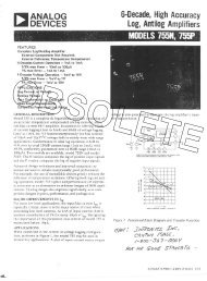
10 kHz. Typical PWM signals produced by the dedicated PWM
generation unit of the ADMC401 are shown in Figure 2, for
inverter leg A. In the figure, AH is the signal used to drive the
high-side power device of inverter leg A, and AL is used to drive
the low-side power device. The duty cycle effectively adjusts the
average voltage applied to the motor on a cycle-by-cycle basis to
achieve the desired control objective.
In general, there is a small delay required between turning off one
power device (say AL) and turning on the complementary power
device (AH). This dead-time is required to ensure the device being
turned off has sufficient time to regain its blocking capability before
the other device is turned on. Otherwise a short circuit of the dc
voltage could result. The PWM generation unit of the ADMC401
contains the necessary hardware for automatic dead-time insertion
into the PWM signals.
CONTROLLER
INTERRUPTS
AH
AL
CONTROL PERIOD
N
CONTROL PERIOD
N+1
CONTROL PERIOD
N+2
50 100 150 200
DUTY CYCLE, D1 DUTY CYCLE, D2 DUTY CYCLE, D3
TIME
s
Figure 2. Typical PWM waveforms for a single inverter leg.
General Structure of a Three-Phase AC Motor Controller
Accurate control of any motor-drive process may ultimately be
reduced to the problem of accurate control of both the torque and
speed of the motor. In general, motor speed is controlled directly
by measuring the motor’s speed or position using appropriate
transducers, and torque is controlled indirectly by suitable control
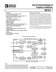
of the motor phase currents. Figure 3 shows a block diagram of a
typical synchronous frame-current controller for a three-phase
motor. The figure also shows the proportioning of tasks between
software code modules and the dedicated motor-control
peripherals of a motor controller such as the ADMC401. The
controller consists of two proportional-plus-integral-plusdifferential
(PID) current regulators that are used to control
the motor current vector in a reference frame that rotates
synchronously with the measured rotor position.
Sometimes it may be desirable to implement a decoupling between
voltage and speed that removes the speed dependencies and
associated axes cross coupling from the control loop. The reference
voltage components are then synthesized on the inverter using a
suitable pulsewidth-modulation strategy, such as space vector
modulation (SVM). It is also possible to incorporate some
compensation schemes to overcome the distorting effects of the
inverter switching dead time, finite inverter device on-state voltages
and dc-link voltage ripple.
The two components of the stator current vector are known as the
direct-axis and quadrature-axis components. The direct-axis current
controls the motor flux and is usually controlled to be zero with
permanent-magnet machines. The motor torque may then be
controlled directly by regulation of the quadrature axis component.
Fast, accurate torque control is essential for high-performance
drives in order to ensure rapid acceleration and deceleration—
and smooth rotation down to zero speed under all load conditions.
The actual direct and quadrature current components are obtained
by first measuring the motor phase currents with suitable currentsensing
transducers and converting them to digital, using an on-chip
ADC system. It is usually sufficient to simultaneously sample just
two of the motor line currents: since the sum of the three currents
is zero, the third current can, when necessary, be deduced from
simultaneous measurements of the other two currents.
The controller software makes use of mathematical vector
transformations, known as Park Transformations, that ensure that
the three-phase set of currents applied to the motor is synchronized
to the actual rotation of the motor shaft, under all operating
conditions. This synchronism ensures that the motor always
produces the optimal torque per ampere, i.e., operates at optimal
efficiency. The vector rotations require real-time calculation of the
sine and cosine of the measured rotor angle, plus a number of
multiply-and-accumulate operations. The overall control-loop
bandwidth depends on the speed of implementation of the closedloop
control calculations—and the resulting computation of new
duty-cycle values. The inherent fast computational capability of
the 26-MIPS, 16-bit fixed-point DSP core makes it the ideal
computational engine for these embedded motor-control
applications.
ANALOG-TO-DIGITAL CONVERSION REQUIREMENTS
For control of high-performance ac servo-drives, fast, highaccuracy,
simultaneous-sampling A/D conversion of the measured
current values is required. Servo drives have a rated operation
range—a certain power level that they can sustain continuously,
with an acceptable temperature rise in the motor and power
converter. Servo drives also have a peak rating—the ability to handle
a current far in excess of the rated current for short periods of
time. It is possible, for example, to apply up to six times the rated
4 Analog Dialogue 34-6 (2000)

current for short bursts of time. This allows a large torque to be
applied transiently, to accelerate or decelerate the drive very quickly,
then to revert to the continuous range for normal operation. This
also means that in the normal operating mode of the drive, only a
small percentage of the total input range is being used.
At the other end of the scale, in order to achieve the smooth and
accurate rotations desired in these machines, it is wise to
compensate for small offsets and nonlinearities. In any currentsensor
electronics, the analog signal processing is often subject to
gain and offset errors. Gain mismatches, for example, can exist
between the current-measuring systems for different windings.
These effects combine to produce undesirable oscillations in the
torque. To meet both of these conflicting resolution requirements,
modern servo drives use 12-to-14-bit A/D converters, depending
on the cost/performance trade-off required by the application.
The bandwidth of the system is essentially limited by the amount
of time it takes to input information and then perform the
calculations. A/D converters that take many microseconds to
convert can produce intolerable delays in the system. A delay in a
closed-loop system will degrade the achievable bandwidth of the
system, and bandwidth is one of the most important figures of
merit in these high-performance drives. Therefore, fast analog-todigital
conversion is a necessity for these applications.
A third important characteristic of the A/D converter used in these
applications is timing. In addition to high resolution and fast
conversion, simultaneous sampling is needed. In any three-phase
motor, it’s necessary to measure the currents in the three windings
of the motor at exactly the same time in order to get an instantaneous
“snapshot” of the torque in the machine. Any time skew (time
delay between the measurements of the different currents) is an
error factor that’s artificially inserted by the means of measurement.
Such a non-ideality translates directly into a ripple of the torque—
a very undesirable characteristic.
The ADC system that is integrated into the ADMC401 provides a
fast (6-MSPS), high-resolution (12-bit) ADC core integrated with
dual sample-and-hold amplifiers so that two input signals may be
sampled simultaneously. (As noted earlier, this allows the
simultaneous value of the third current to be calculated.) The ADC
core is a high-speed pipeline flash architecture. A total of eight
analog input channels may be converted, accepting additional
system or feedback signals for use as part of the control algorithm.
This level of integrated performance represents the state-of-theart
in embedded DSP motor controllers for high-performance
applications.
POSITION SENSING AND ENCODER INTERFACE UNITS
Usually the motor position is measured through the use of an
encoder mounted on the rotor shaft. The incremental encoder
produces a pair of quadrature outputs (A and B), each with a
large number of pulses per revolution of the motor shaft. For a
typical encoder with 1024 lines, both signals produce 1024 pulses
per revolution. Using a dedicated quadrature counter, it is possible
to count both the rising and falling edges of both the A and B
signals so that one revolution of the rotor shaft may be divided
into 4096 different values. In other words, a 1024-line encoder
allows the measurement of rotor position to 12-bit resolution. The
direction of rotation may also be inferred from the relative phasing
of quadrature signals A and B.
It is usual to have a dedicated encoder interface unit (EIU) on the
motor controller; it manages the conversion of the dual quadrature
PID
I* QS
PARK
SVM
PID
VOLTAGE
DECOUPLING
e
–j e
NON-
IDEALITY
CORRECTION
FWM
GENERATION
UNIT
PWM
OUTPUTS
+
–
+
–
–j e
I* DS
d —dt
e
3–>2
TRANSFORM
ADC
SYSTEM
MOTOR
CURRENT
FEEDBACK
PARK
ROTOR
POSITION, e
ENCODER
INTERFACE
UNIT
ENCODER
FEEDBACK
SIGNALS
DSP SOFTWARE
MOTOR CONTROL
PERIPHERALS
Figure 3. Configuration of typical control system for three-phase ac motor.
Analog Dialogue 34-6 (2000) 5

encoder output signals to produce a parallel digital word that
represents the actual rotor position at all times. In this way, the
DSP control software can simply read the actual rotor position
whenever it is needed by the algorithm.
This is all very well, but there is an increasing class of cost-sensitive
servo-motor drive applications with lower performance demands
that can afford neither the cost nor the space requirements of the
rotor position transducer. In these cases, the same motor control
algorithms can be implemented with estimated rather than
measured rotor position.
The DSP core is quite capable of computing rotor position using
sophisticated rotor-position estimation algorithms, such as
extended Kalman estimators that extract estimates of the rotor
position from measurements of the motor voltages and currents.
These estimators rely on the real-time computation of a sufficiently
accurate model of the motor in the DSP. In general, these sensorless
algorithms can be made to work as well as the sensor-based
algorithms at medium-to-high speeds of rotation. But as the speed
of the motor decreases, the extraction of reliable speed-dependent
information from voltage and current measurements becomes more
difficult. In general, sensorless motor control is applicable
principally to applications such as compressors, fans, and pumps,
where continuous operation at zero or low speeds is not required.
Conclusions
Modern DSP-based control of three-phase ac motors continues
to flourish in the market place, both in established industrial
automation markets and in newer emerging markets in the home
appliance, office automation and automotive markets. Efficient
and cost-effective control of these machines requires an appropriate
balance between hardware and software, so that time-critical tasks
such as the generation of PWM signals or the real-time interface
to rotor position transducers are managed by dedicated hardware
units. On the other hand, the overall control algorithm and
computation of new voltage commands for the motor are best
handled in software using the fast computational capability of a
DSP core. Implementing the control solution in software brings
all the advantages of easy upgrading, repeatability, and
maintainability, when compared with older hardware solutions.
All motor-control solutions also require the integration of a suitable
A/D conversion system for fast and accurate measurement of the
feedback information from the motor. The resolution, conversion
speed, and input sampling structure of the ADC system need to
be strictly targeted to the requirements of specific applications.
b
Mixed-Signal Motor Control Signal Chain
ADMC300/ADMC330 SINGLE CHIP MOTOR CONTROL IC
DSP CARE
ADSP-21xx
MEMORY
BLOCK
PROGRAMMABLE
I/O
PWM
V REF
ADC
POWER
STAGE
MOTOR CURRENT
FEEDBACK
MOTOR
E
ENCODER OR
RESOLVER
FEEDBACK
R
ENCODER
INTERFACE
OTHER
PERIPHERALS
INTERFACE
R5-232, R5-485
RESOLVER-TO-DIGITAL
CONVERTER
SPEED/DIRECTION/POSITION
COMMAND
COMPUTER
HOST
OSCILLATOR
BUFFER
NOTE:
SELECT THE BLUE SIGNAL CHAIN SM BLOCKS OR THE
BLUE TEXT TO SEE A LISTING OF AVAILABLE PRODUCTS.
Using Mixed-Signal Motor Control ICs
6 Analog Dialogue 34-6 (2000)

Embedded Modems
Enable Appliances
to Communicate with
Distant Hosts via the
Internet
by Rick Blessington
Software & Systems Technology Division*
INTRODUCTION
Today’s smart appliances do much more than shut off the dryer
when the clothes are dry or display a new photograph when one
has been shot. For example: they provide status information
indicating when a vending machine needs to be filled or a drop
box emptied; they run remote diagnostics when needed, and
automatically upgrade their settings and download software
upgrades to stay current; they schedule and request maintenance
to avoid malfunctions; they add intelligence to the appliances that
harbor them.
Any equipment that does not require an embedded PC, but relies
on data or fax to communicate with a remote host, is likely to
require an embedded modem. Internet appliances designed solely
to provide information via email or the Web need embedded
modems to provide the communications link to the Internet. Settop
boxes for interactive cable and satellite television require
embedded modems to communicate billing information,
interactive programming, pay-per-view, and home shopping orders.
Appliances and handheld computers (or PDAs) become much
more useful when they can link to remote hosts.
The Handspring Visor, for example, can maintain schedules and
calendars, contact lists and telephone directories, expense logs and
time sheets, stock portfolios, and sports team statistics. To be
completely useful, however, the information must be both current
and identical to the information in the user’s computer, company
database, and administrative assistant’s office tools and paper files.
With its Springboard modem, from card access, which uses an
Analog Devices embedded modem chipset, the Visor can be
connected to a telephone line and automatically update both itself
and its user’s host computer. In this way, the Visor becomes the
accurate, timely, and functional information appliance its users
need. Its embedded modem makes all of these capabilities possible
by linking it to a remote host without loading the PDA, because of
the Analog Devices DSP used in the embedded modem.
The Visor required its modem to have low power, small size, high
reliability, standalone form factor, and ease of Internet interfacing.
The resulting Springboard modem fits entirely inside the Visor
package, operates from the Visor’s existing batteries without
significantly shortening their life, and automatically connects to
the Internet when connected to a telephone line. It makes the
Visor an extension of its user’s computer network.
Embedded Modem Components
Embedded modems contain a data pump, DAA (data access
arrangement), and modem code. They may or may not include a
controller, Internet protocol stack, and SDRAM. The number of
chips depends on the application requirements, including the need
for any additional functions. They connect to telephone lines, and
include all the necessary hardware and software.
A data pump includes a processor (DSP) that translates data to a
standard protocol (fax or Internet), at a specific bit rate, such as
V.32, V.34, V.90, employing modem code. A DAA provides the
physical and software interface to a POTS (plain old telephone
service) line. A silicon DAA performs this function without external
codecs, relays, optocouplers, and transformers. An Internet protocol
(IP) stack implements the Internet protocols (such as PPP, TCP,
HTTP, POP3, FTP, etc.) on the modem’s DSP. This permits file
downloads, standard Web-page hosting, and email capability for
the device to which the modem is connected without the use of a PC,
microcontroller, or other processor. Thus the DSP executes both the
modem code and the IP stack.
Modem Architecture Trade-Offs
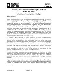
Embedded modems may be either controller-based (parallel) or
operate without a controller. In both cases they need a fixed-point
DSP data pump and DAA. The modem code can either run on
the DSP data pump, or on a Pentium ® or RISC processor (for
host-based or software modems), or on a multifunction
programmable DSP (such as an ADSP-218x). For comparison,
modem architectures may be divided into two host-based classes
(with and without on-board processing), and two standalone classes
(microcontroller- and DSP-based). Their characteristics and
advantages/disadvantages are compared in Table I.
The controller-based designs work without hosts, so they don’t care
about operating systems or whether the host has crashed. This
standalone approach assures greater redundancy, since the modem
operates independently of the host computer and its operating
system. Their downside is they need a microcontroller and its
memory, as well as DSP memory, to run the supervisory code.
This entails additional parts count, real estate and power, and
consequently added cost and risk. Also, their modem software is
usually hard-coded and consequently not upgradeable.
DTE
MICRO-
CONTROLLER
MEMORY
SUPERVISORY
CODE
DATA PUMP
SRAM
MODULATION
CODE
Figure 1. Controller-based modem.
DAA
TELCO
*For more details, contact willie.waldmann@analog.com or
ajai.gambhir@analog.com.
Analog Dialogue 34-7 (2000) 7

Table I. Modem Architecture Overview
Type Controller-Based— Controllerless—Serial Multifunction
Trade-Offs (+ and –) Parallel (or Winmodem) Software—Host-Based Programmable—DSP-Based
Requires Host No Yes Yes No
Redundancy Best. Stays alive None. Relies on host. None. Relies on host. Best. Stays alive when host
when host crashes.
crashes.
Upgradeability None Depends on host. Least Best
Cost Most Moderate Lowest Moderate
Downside(s) Needs microcontroller Needs host to run Requires more power. Ongoing price competition
with memory to run supervisory code. Data Limited to Pentium and with host-PC pricing erosion.
supervisory code. pump still needs memory. Windows applications.
Uniqueness Operating-system Memory resides on Software only. No host or operating system
neutral host. Supervisory code and dependencies. Integrated
DSP runs on host. controller and data pump.
Controllerless (software-controlled, or win-) modems, offer lower cost,
real estate, and power since the memory resides on the PC and no
microcontroller (nor memory for it) is needed. However, they
require a PC to run the supervisory code, so these winmodems
are heavily dependent on the PC operating system. Consequently,
uptime of the PC host is important to their operation, and they
are affected by the typical PC install/support issues. Their
performance suffers when the host is heavily loaded with other
jobs. They still require a data pump with memory. Code upgrades
and diagnostics are dependent on the reliability of the PC host,
with no redundancy. Software upgrades are limited by the modem’s
fixed amount of memory.
PERSONAL
COMPUTER
DRAM
SUPERVISORY
DATA PUMP
SRAM
MODULATION
DAA
ISOLATION
Figure 2. Controllerless modem (ISA and PCI).
TELCO
Software, host-based or soft-modems operate without a DSP or
microcontroller, since their supervisory and data pump code runs
on the PC host. This approach has been promoted by PC processor
manufacturers to take advantage of the “free” unused MIPS of
the increasingly more powerful host processors, since the modems
do not significantly load the host, but at the same time they help
justify the need to upgrade to it. These modems are very low cost
because they use the existing host. On the other hand, if the cost
of upgrading to a sufficiently fast host to handle the modem
functions is taken into consideration, the result will far surpass
the cost of either a controller-based or controllerless design. Hostbased
modems are also heavily dependent on their host’s reliability,
as well as concurrency issues encountered when running many
operations simultaneously. In addition, this approach typically
limits the modem to communicating only Windows and Pentium
applications, limiting the “free” MIPS (millions of instructions
per second) on the host to particular functions. The power drain
and cost-per-MIPS for a Pentium is much higher than for a DSPbased
design, so the power used by the board must be taken into
account, even if the cost is not. The cost of modem IP must still be
paid, so the concept of “free” is not accurate.
A multifunction DSP-based embedded modem incorporates a
programmable DSP, such as an ADSP-218x. By integrating the
controller, memory, and data pump on a single chip, real estate
(board space), cost, and power are reduced. No separate
microcontroller or associated memory is required. A software-based
UART is used, further reducing the hardware cost, real estate,
and power. The standalone design operates independently of the
host and operating system, offering redundancy and remote
software upgradeability via the included FLASH memory. The
codec adds international capabilities, accommodating countryspecific
parameters. Three modulation speeds are possible, each
using the same components but a different Internet protocol (IP):
up to 14.4 kbps, up to 33.6 kbps and up to 56 kbps.
The Analog Devices programmable DSP-based embedded
modems capture the advantages of all the above approaches with
few of their disadvantages. Even as PC prices fall while host PC
performance increases, embedded DSP MIPS will always remain
less expensive, more reliable, and independent of host processing.
RS232/TTL
SERIAL OR
IDMA
PARALLEL
PROGRAM
SRAM
ADDST
218x
FLASH
(OR SYSTEM)
MEMORY
SOFTWARE
BY
TELINDUS
DATA
SRAM
DIGITAL
ISOLATION
SIDE
SILICON DAA
LINE
SIDE
RJ11
TELCO
Figure 3. Multifunction DSP-based modem.
All of the alternatives, except the host-based design, have the
disadvantage of facing competition with continuing PC host price
erosion. As the PC host price decreases relative to that of the standalone
modem, host-based modems become more cost effective. The
trade-off between redundancy and cost, however, will continue.
8 Analog Dialogue 34-7 (2000)

DAA Approaches
The DAA (data access arrangement) supports country-specific
Call Progress and Caller ID, which must be specified for each
country. Different DAA components are available to support
worldwide operation of a subset of countries. The DAA handles
TIP and RING telephone connections—and includes a second
codec for nonpowered lines, such as leased lines and wireless.
Multiple DAAs can be supported by a single DSP for use in multiline
applications.
The state-of-the-art international silicon DAA with integral codec
eliminates the cost and real estate of transformers, optoisolators,
relays, and hybrids. All of this is replaced with two small TSSOP
packages that directly connect to the DSP, improving reliability
and manufacturing ease while decreasing real estate and cost. The
design improves performance, since the signals are digitally
transmitted over the isolation barrier. The silicon DAA includes
international support in a single design and supports both U.S.
and international caller ID without relays, via software
programmability, for different countries. No hardware modification
is required. Advanced power management, caller ID, and sleep mode
save power and offer green compliance, enabling a smaller power
supply and longer battery life. Monitor output and microphone
input support voice and handset applications.
Each modem design also supports legacy DAAs used for unpowered
telephone line applications, such as wireless and leased lines.
Software Development
Analog Devices’ embedded modems include modem code
supplied by Telindus. Product-specific software can be obtained
from modem partners of Analog Devices. For example, one can
automatically link the Handspring Visor to the Internet by adding
a Springboard modem from Card Access. One can enable a
Lavazza e-espressopoint coffee machine to send and receive
emails (to trigger maintenance checks and restocking visits, and
display weather or traffic reports) by adding an Internet modem
from Analog Devices that executes a TCP/IP stack from eDevice.
Modem Reference Designs
The Analog Devices embedded modem development platform
includes an ADSP-218x programmable DSP and a silicon DAA.
It consumes under 200 mW maximum power at 3.3 V. No customer
code is required. The development platform includes modem
software from ISO 9001-certified Analog Devices’ technology
partner Telindus. The board comes with connectors for EZ-ICE,
JTAG, and RS-232 I/O for modification and testing of the AT
command set and S registers.
Embedded Modem Applications
The products that use embedded modems for communication
include vending machines (which can communicate levels of
inventory and when they need to be filled), kiosks, POS terminals,
security and surveillance systems, games, and drop boxes that can
communicate when they have shipments to be picked up. The ways
in which the basic product communicates via these standalone
modems are established by programming in relevant web content
and communication data. The results for designers are products
with such characteristics as built-in investment protection,
appliances that “know” and communicate when they need to be
serviced, fixed, filled, emptied, updated, or picked up. Products
that use the Internet to provide customer information and
communications can be located wherever needed. Industrial
equipment can indicate when it needs to be serviced. Refrigerators
can display recipes containing only the ingredients on their shelves.
Standalone embedded modems can reduce operating costs at the
same time that they make possible new product categories with
features to spur new sales. With new Internet-enabled power, these
products can create new opportunities for e-commerce, e-service,
and e-information vendors.
Standalone embedded modems offer complete and flexible design
alternatives for worldwide communications in a variety of
approaches. Each approach can be configured on as few as three
chips, offers a choice of speeds, and can be implemented
inexpensively with low power and real estate requirements.
Embedded modems can bring the power of Internet information
and communications to both new and installed devices and can add
automatic software upgrades and remote diagnostics at the same time.
For Further Information
For additional help, contact systems.solutions@analog.com, or
visit Analog Devices Software & Systems Technologies on the Web.
Or contact Analog Devices’ modem partners: Card Access
and eDevice.
b
ISOLATION
TOP VIEW
ONLY
1 INCH!
DSP
BOTTOM VIEW
DAA
RS-232
TRANSCEIVER
TTL LED DRIVER
FLASH
ONLY 2 1/2 INCHES!
Figure 4. V.90 standalone embedded modem reference design.
Analog Dialogue 34-7 (2000) 9

Adaptively Canceling
Server Fan Noise
Principles and Experiments with
a Short Duct and the AD73522
dspConverter
by Paschal Minogue, Neil Rankin, Jim Ryan
INTRODUCTION
In the past, when one thought of noise in the workplace, heavy
industrial noise usually came to mind. Excessive noise of that type
can be damaging to the health of the worker. Today, at a much
lower level, though not as severe a health hazard in office
environments, noise from equipment such as personal computers,
workstations, servers, printers, fax machines, etc., can be
distracting, impairing performance and productivity. In the case
of personal computers, workstations and servers, the noise usually
emanates from the disk drive and the cooling fans.
This article is about the problem of noise from server cooling fans,
but the principles can be applied to other applications with similar
features. Noise from server cooling fans can be annoying, especially
when the server is located near the user. Usually, greater server
computing power means higher power dissipation, calling for
bigger/faster fans, which produce louder fan noise. With effective
fan noise cancellation, bigger cooling fans could be used, permitting
more power dissipation and a greater concentration of computer
power in a given area.
A block diagram of a basic ANC system as applied to noise
propagating inside a duct is illustrated in Figure 2. The noise
propagating down the duct is sampled by the upstream reference
microphone and adaptively altered in the electronic feed-forward
path to produce the antinoise to minimize the acoustic energy at
the downstream error microphone. However, the antinoise can
also propagate upstream and can disrupt the action of the adaptive
feedforward path, especially if the speaker is near the reference
microphone (as is always the case in a short duct). To counteract
this, electronic feedback is used to neutralize the acoustic feedback.
This neutralization path is normally determined off-line, in the
absence of the primary disturbance, and then fixed when the
primary noise source is present. This is done because the primary
noise is highly correlated with the antinoise.
There are many problems associated with short-duct noise
cancellation [2, 3, 4]. Acoustic feedback from antinoise speaker to
reference microphone is more pronounced; the number of acoustic
modes increases exponentially; duct resonances can cause
harmonic distortion; and the group delay through the analog-todigital
converters, processing unit, and digital-to-analog converters
can become significant [5]. This paper concentrates on the latter
problem in particular.
DUCT
REFERENCE
MICROPHONE
FIXED
FIR
(FEEDBACK)
ANTINOISE
SPEAKER
ERROR
MICROPHONE
+
–
Figure 2. Basic duct ANC system.
DESCRIPTION OF PROBLEM
Typically, server cooling-fan noise has both a random and a
repetitive component. A spectrum plot of the fan noise of the Dell
Poweredge 2200 server illustrates this (Figure 1). Also, the profile
of the fan noise can change with time and conditions; for example,
an obstruction close to the fan will affect its speed and thus the
noise that it generates.
PROGRAMMABLE
FIR
(FEEDFORWARD)
LMS
UPDATE
ALGORITHM
AMPLITUDE – dB
0
THE IMPORTANCE OF GROUP DELAY
To provide an unobtrusive and viable solution in terms of size and
cost, the smaller the duct is made the better; ideally, it should fit
inside the server box—which would result in a very short acoustic
path. To maintain causal relationships, the delay through the entire
(mostly electronic) feedforward path has to be less than or equal
to the delay in the forward acoustic path if broadband primary
noise is to be successfully cancelled.
δ
ff
≤ δ
(1)
ap
–70
0 10
FREQUENCY – kHz
Figure 1. Profile of server fan noise.
ONE SOLUTION
One solution is to confine the propagation of much of the fan
noise to a duct, and then use active noise control (ANC) to reduce
the strength of the fan noise leaving the duct [1].
where δ ff is the delay through the feedforward path and δ ap is the
primary acoustic delay.
In cases where the secondary speaker is recessed into its own short
duct, the feedforward path will also include the acoustic delay
through this secondary duct.
δ ff = δ e + δ as (2)
where δ e is the electronic part of the feedforward path and δ as is
the acoustic delay in the secondary duct.
10 Analog Dialogue 34-2 (2000)

The electronic delay in the feedforward path consists of group
delay through the microphone, anti-aliasing filter and A/D
converter (ADC); processing delay (+ digital filter group delay) in
the DSP; group delay through the D/A converter (DAC) and antiimaging
filter; and finally the delay through the secondary speaker.
δ e = δ mic + δ adc + δ dsp + δ dac + δ spkr (3)
Therefore, from causality:
δ mic + δ adc + δ dsp + δ dac + δ spkr + δ as ≤ δ ap (4)
To minimize δ ap , and thereby the length of the duct, δ ff (and all its
various components) should be made as small as possible. Let’s
assume that delays through the microphone, speaker and secondary
duct path have already been minimized. Then, the remaining
quantity to be minimized is δ adc + δ dsp + δ dac .
δ adc can be minimized by using an oversampled ADC with low
group-delay-decimation filtering; δ dsp can be minimized by using
a DSP with sufficiently high-MIPS and an efficient instruction
set; δ dac can be minimized by using an oversampled DAC with
interpolation filtering having low group delay. The latter should
be capable of being bypassed to further minimize the group delay.
Furthermore, the processor should use the most recent ADC
sample as soon as it becomes available, and the DAC should use
the latest DSP output result as soon as it becomes available. To
achieve this, it must be possible to advance the timing of the DAC
relative to the ADC in some fashion.
High-speed gain taps in parallel with the main processing path
can help to ease the situation, especially in the case of practical
short ducts where the noise can flank the acoustic path via the
duct hardware itself.
Although a feedforward cancellation technique with a very low
group delay is required to cancel the random component when
using a relatively short duct, a feedback approach can be applied
to cancel the repetitive component using an rpm sync signal as
the reference input.
ANC ARCHITECTURE
Less group delay through the cancellation system means that a
shorter duct can be used, making the approach more feasible and
acceptable. To achieve very low group delay, a heavily oversampled
sigma-delta converter technique is employed at the analog frontend
(AFE) section of the system. Furthermore, both an analog
gain tap (AGT) and a digital gain tap (DGT) can be utilized to
provide even lower group delay in the processing path.
With no high-speed gain taps, a 2-ADC/1-DAC configuration
(Figure 3) can be used, as all the processing is done digitally and
at a relatively low rate. In Figure 3, each conversion channel is
shown with its sample-rate conversion in a separate block: a
decimator block in the case of the ADC channel and an interpolator
block for the DAC channel.
ADC
DEC
REFERENCE
MICROPHONE
+
–
DUCT
FIXED
FIR
(FEEDBACK)
PROGRAMMABLE
FIR
(FEEDFORWARD)
LMS
UPDATE
ALGORITHM
ANTINOISE
SPEAKER
DAC
INT
ADC
DEC
ERROR
MICROPHONE
Figure 3. A 2-ADC/1-DAC configuration with no highspeed
gain taps.
The introduction of gain taps is illustrated in Figure 4. Filters
with gain taps can be thought of as just single-tap FIR filters. The
feedforward tap is programmable and adapted during cancellation;
the feedback tap is fixed and determined off-line.
Note that the DGTs act on the high-rate output of the ADC and
their outputs are combined with the high-rate input to the DAC.
ADC
DEC
REFERENCE
MICROPHONE
PROGRAMMABLE
FIR
(FEEDFORWARD)
LMS
UPDATE
ALGORITHM
DUCT
ANTINOISE
SPEAKER
+ –
FIXED GAIN TAP
(FEEDBACK)
+ –
FIXED
DAC INT FIR DEC ADC
(FEEDBACK)
PROGRAMMABLE
GAIN TAP
(FEEDFORWARD)
INT
DAC
+ +
ADC
DEC
ERROR
MICROPHONE
Figure 4. ANC system with high-speed analog and digital
gain taps.
Analog Dialogue 34-2 (2000) 11

ANC ALGORITHM
The standard filtered-x LMS (FXLMS) algorithm was used to
update the ANC coefficient for the feedforward cancellation,
h k+1 = h k + 2 µ × e k × x' k (5)
where x' k is filtered by the secondary path model. Other adaptive
algorithms have been suggested for improved performance on
fixed-point DSPs [6].
The modeling for the secondary path and feedback neutralization
path is done off-line; then fixed versions are used in the activecancellation
mode. In addition, each microphone input is processed
through an adaptive dc tap, and a leakage component is optionally
part of the feedforward-path coefficient update algorithm.
ANC HARDWARE AND SOFTWARE REQUIREMENTS
The short-duct ANC hardware should include an AFE with at
least two ADC channels and one DAC channel. The reference
signal ADC and the antinoise DAC need to have inherently high
sample rates and low group delay. The sampling timing of the
antinoise DAC should be capable of being advanced relative to
the sample timing of the reference ADC. The AFE should also
have both high-speed analog and digital gain taps to provide an
ultra-short delay path. The error-signal ADC also needs to be low
in group delay, as its delay contributes to the delay through the
secondary path as seen by the processor from the antinoise speaker
to the error microphone. As this secondary path model has to be
run by the processing block as well as the main feedforward path,
it should be as short as possible. The main processing block should
have as high a MIPS rate as possible (with an efficient instruction
set) to reduce the delay, keeping within the general requirement
for a low-cost solution. Finally, a single-package embodiment of
the main signal conversion and processing functions should make
the ANC solution more flexible yet cost-effective.
One such ANC solution with a single integrated circuit package
can be obtained using the AD73522 dspConverter.
AD73522 PRODUCT INFORMATION
The AD73522 (Figure 5) is a single-device dspConverter
incorporating a dual analog front end (AFE), a microcomputer
optimized for digital signal processing (DSP) and a flash-based
boot memory for the DSP.
The AFE section features two 16-bit ADC channels and two
16-bit DAC channels. Each channel provides 77-dB signal-to-noise
ratio over a voiceband signal bandwidth with a maximum sample
rate of 64 ksps. It also features an input-to-output gain network in
both the analog (AGT) and digital (DGT) domains. The low
group-delay characteristic (typically 25 µs per ADC channel and
50 µs per DAC channel) of the AFE makes it suitable for singleor
multi-channel active control applications. The ADC and DAC
channels feature programmable input/output gains with ranges of
38 dB and 21 dB respectively. An on-chip reference voltage is
included to allow single-supply operation.
The AD73522’s 52-MIPS DSP engine combines the ADSP-2100
family base architecture (three computational units, data address
generators and a program sequencer) with two serial ports, a
16-bit internal DMA port, a byte DMA port, a programmable
timer, flag I/O, extensive interrupt capabilities, and on-chip
program- and data memory.
The AD73522-80 integrates 80 Kbytes of on-chip memory
configured as 16K 24-bit words of program RAM and 16K 16-bit
words of data RAM. The AD73522-40 integrates 40K bytes of
on-chip memory configured as 8K words of 24-bit program RAM
and 16-bit data RAM.
Both devices feature a Flash memory array of 64 Kbytes
(512 Kbits) connected to the DSP’s byte-wide DMA port
(BDMA). This allows nonvolatile storage of the DSP’s boot code
and system data parameters. The AD73522 runs from a 3.3-V
power supply. Power-down circuitry is inherent to meet the lowpower
needs of battery-operated portable equipment.
POWER-DOWN
CONTROL
ADC1
REF
DATA ADDRESS
GENERATORS
DAG 1 DAG 2
PROGRAM
SEQUENCER
18K PM
(OPTIONAL 8K)
MEMORY
18K DM
(OPTIONAL 8K)
PROGRAMMABLE
I/O
AND FLAGS
FULL MEMORY
MODE
DAC1
SERIAL
PORT
PROGRAM MEMORY ADDRESS
DATA MEMORY ADDRESS
PROGRAM MEMORY DATA
EXTERNAL
ADDRESS
BUS
EXTERNAL
DATA
BUS
ADC2
SPORT 2
DATA MEMORY DATA
BYTE DMA
CONTROLLER
ARITHMETIC UNITS
SERIAL PORTS
TIMER
DAC2
ALU MAC SHIFTER
ADSP-2100 BASE
ARCHITECTURE
SPORT 0 SPORT 1
FLASH
BYTE MEMORY
64K BYTES
ANALOG FRONT END
SECTION
Figure 5. AD73522 dspConverter.
12 Analog Dialogue 34-2 (2000)

VFBN1
VINN1
VINP1
VFBP1
V REF
+
+
+
GAIN
1
INVERT
SINGLE-ENDED
ENABLE
+
0/38dB
PGA
–
ANALOG
SIGMA-DELTA
MODULATOR
+
GAIN
1
DECIMATOR
VOUTP1
VOUTN1
+ CONTINUOUS
+6/–15dB TIME
PGA LOW-PASS
FILTER
SWITCHED
CAPACITOR
LOW-PASS
FILTER
1-BIT
DAC
DIGITAL
SIGMA-
DELTA
MODULATOR
INTERPOLATOR
Figure 6. Analog front-end subsection of the AD73522 dspConverter.
SIGMA-DELTA ADC AND DAC ARCHITECTURE
The conversion technique adopted in the AFE is of the sigmadelta
type. An analog sigma-delta modulator is used in the ADC
channel and a digital sigma-delta modulator is employed in the
DAC channel. A sigma-delta modulator is a heavily oversampled
system that uses a low-resolution converter in a noise-shaping loop.
The quantization noise of the low-resolution, high-speed converter
is inherently high-pass filtered and “shaped” out of band. The
output of the modulator or noise shaper is then low-pass filtered
to reduce the sample rate and remove the out-of-band noise.
The AFE conversion channels used in the AD73522 are shown in
Figure 6. The ADC section consists of an analog second-order,
32× to 256× oversampling, 1-bit sigma-delta modulator, followed
by a digital sinc-cubed decimator (divide-by-32 to divide-by-256).
The DAC section contains a digital sinc-cubed interpolator, a
digital, second-order, 32× to 256× oversampling, 1-bit sigma-delta
modulator, followed by an analog third-order switched-capacitor
LPF and a second-order continuous-time LPF.
The group delay through the ADC channel is dominated by the
group delay through the sinc-cubed decimator and is given by the
following relationship:
M − 1
δdec
= Order × × δds
(6)
2
where Order is the order of the decimator (= 3), M is the decimation
factor (= 32 for 64-ksps output sample rate) and δ ds is the
decimation sample interval (= 1/2.048E6 s)
32 – 1 1
⇒ δ dec = 3 × ×
2 2.
048E6
⇒ δ dec = 22.7 µs
for a 64-ksps output sample rate.
The group delay through the DAC channel is primarily determined
by the group delay through the sinc-cubed interpolator and the
group delay through the third-order switched-capacitor LPF. The
inherent group delay through the interpolator is identical to that
through the decimator and equals 22.7 µs for 64-ksps input sample
rate. However, the interpolator can be optionally bypassed to
(7)
avoid this inherent group delay at the expense of reduced outof-band
rejection.
The z-transform of both the sinc-cubed decimator and interpolator
is given by:
3
⎡ – M
1 – z ⎤
⎢
– 1
⎥
(8)
⎣⎢
1 – z ⎦⎥
The group delay through the analog section of the DAC is
approximately 22.7 µs.
Notice that with sample rates of only 8 ksps the inherent group
delays through both the decimator and interpolator increase to
186.8 µs. Therefore, it is very important to run the converters at
as high a rate as possible to reduce the inherent group delay.
The AFE features high-speed analog and digital feedforward paths
from ADC input to DAC output via the AGT and DGT
respectively. The AGT is configured as a differential amplifier with
gain programmable from –1 to +1 in 32 steps and a separate mute
control. The gain increment per step is 0.0625. The group delay
through the AGT feedforward path is only 0.5 µs. The DGT is a
programmable gain block whose input is tapped off from the bitstream
output of the ADC’s analog sigma-delta modulator. This
single-bit input is used to add or subtract the digital gain tap setting,
a 16-bit programmable value, to the output of the DAC’s
interpolator. The group delay through the DGT feedforward path
is only 25 µs.
The loading of the DAC is normally internally synchronized with
the unloading of the ADC data in each sampling interval. However,
this DAC load position can be advanced in time by up to 15 µs in
0.5-µs steps. This facility can be used to further minimize the
feedforward delay from analog input to analog output via the DSP.
AD73522 PACKAGING
The three main processing elements (AFE, DSP and Flash
memory) are combined in a single package to give a cost-effective,
self-contained solution. This single package is a 119-ball plastic
ball grid array (PBGA), as shown in Figure 7. It measures 14 mm
× 22 mm × 2.1 mm, and the solder balls are arranged in a 7 × 17
array with a 1.27-mm (50 mil) pitch.
Analog Dialogue 34-2 (2000) 13

TOP VIEW
14 mm
user-friendly programming platform that allows quick and easy
development. The board, interfacing to the serial port of a PC,
comes with Windows ® 95-compatible interface software that allows
the transfer of data to and from all memory, including the Flash
sections. All of the dspConverter pins are available at the output
connectors. The board has an EZ-ICE ® connector for advanced
software development. Other features include a microphone with
conditioning circuitry on one input channel and speaker amplifiers
on the output channels.
22 mm
a.
BOTTOM VIEW
Figure 8. AD73522 dspConverter evaluation board.
7 ROWS 17 COLUMNS OF SOLDER BALLS
b.
Figure 7. AD73522 plastic ball grid array (PBGA) packaging.
AD73522 EVALUATION BOARD
The AD73522 dspConverter evaluation board (Figures 8 and 9)
combines all of the front-end analog signal conditioning with a
EXPERIMENTAL SETUP
The experimental setup (Figure 10) consists of a server box
(containing just a fan and power supply), a plastic duct (with
reference and error microphones and secondary loudspeaker), and
the AD73522 evaluation board. The server fan was 5 inches (about
13 cm) in diameter. The T-shaped duct and the speaker measured
6 inches (about 15) cm in diameter. The duct length was adjustable
down to a minimum of 12 inches (30.5 cm).
SWITCHES
512k 8
FLASH
EZ-ICE
J1
RESET
LED
DATA
D7–D0
DATA
D15–D0
ADDRESS
A13–A0
D20–D16
FLAGS AND SPORT
J13
12V DC
5V DC
J10
J11
POWER
CIRCUITRY
INTERRUPT
DVCC
3.2V
LED
PF7
FL1
AD73422/
AD73522
ADDRESS/DATA/CONTROL
PF3
FL0
RS-232
DRIVER
SPORT 0
J12
J3
J2
PC
INTERFACE
MIC
INPUT
(1)
INPUT
(2)
J9
J8
J4
AVCC
3.2V
CH1 CH2 CH1 CH2
INPUT
CONDITIONING
CIRCUITRY
PF4
OUTPUT
CONDITIONING
CIRCUITRY
dspCONVERTER EVALUATION BOARD
POWER
AMP
J7
J5
J6
8
SPEAKER
OUT
OUTPUT
(1)
OUTPUT
(2)
Figure 9. Block diagram of the AD73522 dspConverter evaluation board.
Windows is a registered trademark of Microsoft Corporation.
EZ-ICE is a registered trademark of Analog Devices, Inc.
14 Analog Dialogue 34-2 (2000)

During experimentation, the AD73522 evaluation board was
hooked up to a PC for debug. Also, internal variables were written
out to unused DAC channels for monitoring. Initially, the system
was set up using a primary speaker instead of the actual server fan
to allow testing with programmable tones and broadband signals.
AMPLITUDE – dB
0
ANC
NO ANC
–60
0.2
FREQUENCY – kHz
0.6
Figure 12. Performance with broadband disturbance.
Figure 10. Server fan experimental setup.
RESULTS
The performance of the experimental setup with a single-tone
disturbance from the primary speaker is shown in Figure 11. The
main tone is reduced by a factor of 30 dB. When the primary
speaker delivers a broadband disturbance, the reduction factor is
about 20 dB, as illustrated in Figure 12.
AMPLITUDE – dB
0
NO ANC
CONCLUSIONS
An approach combining an analog gain tap (AGT) and digital
gain tap (DGT) allows the use of sigma-delta techniques in lowgroup-delay
ANC applications. A single-package embodiment
combining analog and digital functions, like the AD73522
dspConverter, should provide an ANC solution that is both flexible
and cost-effective.
ACKNOWLEDGEMENTS
Dell Computer, Limerick, Ireland, for the Poweredge 2200 server
box used in the experimental setup.
Cork Institute of Technology, Cork, Ireland, for the duct
construction used in the experimental setup and a kick-start in
the code development.
The Institute of Sound and Vibration Research (ISVR) and
Digisonix, Inc., for an excellent introduction to active noise control.
ANC
–80
0 1
FREQUENCY – kHz
a. 136-Hz performance, with and without ANC.
AMPLITUDE – dB
0
NO ANC
ANC
–80
0 1
FREQUENCY – kHz
b. 510-Hz performance, with and without ANC.
Figure 11. Noise spectra with single-tone disturbance.
REFERENCES
1. S.M. Kuo & D.R. Morgan, Active Noise Control Systems:
Algorithms and DSP Implementations (Wiley, New York, 1996)
2. “A Primer on Active Sound and Vibration Control,” L.J.
Eriksson, Digisonix brochure
3. “Application of Active Noise Control for Small-Sized Electronic
Equipments,” T. Hoshino, K. Fujii, T. Ohashi, A. Yamaguchi,
H. Furuya, J. Ohga, Inter-noise 94, 1409-1412 (1994)
4. “Study of Active Noise Control System for Duct with High
Speed Flow,” T. Hoshino, T. Ohashi, J. Ohga, H. Furuya, A.
Yamaguchi, K. Fujii, Active95 (International Symposium on
Active Control of Sound and Vibration), 423-430 (1995)
5. “Active Control of Fan Noise in a Personal Computer,” M.
O’Brien, P. Pratt, IEEE ISSC 99 Digest, pp. 385-392 (1999)
6. “An Adaptive Algorithm for Active Noise Control System by a
Fixed Point Processing Type DSP,” K. Fujii, A. Yamaguchi, H.
Furuya, J. Ohga, Active97, 1163-1170 (1997)
7. “Short Duct Server Fan Noise Cancellation,” P. Minogue, N.
Rankin, J. Ryan, Active99, 539-550 (1999) b
Analog Dialogue 34-2 (2000) 15

Fan-Speed Control
Techniques in PCs
by David Hanrahan
Analog Devices offers a comprehensive set of hardware-monitoring
products for use in desktop and notebook PCs and servers.
Intelligent systems-monitoring devices make possible sophisticated
fan speed control techniques to provide adequate cooling and
maintain optimal thermal performance in the system. During the
past year a family of products has been developed, including the
ADM1029 Dual PWM Fan Controller and Temperature Monitor,
the ADM1026, and ADM1030/ADM1031 Complete, ACPI-
Compliant, Dual-Channel ± 1°C Remote Thermal Monitor with
integrated fan controller for one or two independent fans. They
build on the core technology used in the ADM102x PC System
Monitor product portfolio (see also Analog Dialogue 33-1 and 33-
4). Providing fan speed control based on the temperatures
measured within the system, these new products offer more
complete thermal-management solutions. We discuss here the need
for this level of sophisticated control and the issues inherent in
providing it.
BACKGROUND
As the new millennium dawns, processors are achieving speeds of
1 GHz and more. Their impressive improvements in speed and
system performance are accompanied by the generation of
increasing amounts of heat within the machines that use them.
The need to safely dissipate this heat, along with moves in the
computing industry to develop “Green PCs” and user-friendly
machines (as Internet appliances become mainstream), has driven
the need for, and development of, more sophisticated cooling and
thermal management techniques.
PCs have also begun to become smaller and less conventional in
size and shape—as can be seen in any of the latest concept PCs or
slim-line notebooks on the market. Rigid power dissipation
specifications such as “Mobile Power Guidelines ’99” (Ref. 1)
stipulate how much heat may be safely dissipated through a
notebook’s keyboard without causing user discomfort. Any excess
heat must be channeled out from the system by other means, such
as convection along heat pipes and a heat-spreader plate, or the
use of a fan to move air through the system. Clearly, what is needed
is an intelligent, effective approach to thermal management that
can be universally adopted. Various industry groups have assembled
to address these and other issues, and have developed standards
such as ACPI (advanced configuration and power interface) for
notebook PCs and IPMI (intelligent platform management interface)
for server management.
INDUSTRY STANDARDS
The development of the new thermal management/speed control
products was motivated by the ACPI and IPMI standards.
The Advanced Configuration and Power Interface—ACPI (Ref 2) was
defined by Intel, Microsoft, and Toshiba primarily to define and
implement power management within notebook PCs.
Power management (Ref. 2) is defined as “Mechanisms in
hardware and software to minimize system power consumption,
manage system thermal limits, and maximize system battery life.
Power management involves trade-offs among system speed, noise,
battery life, processing speed, and ac power consumption.”
Consider first a notebook-PC user who types trip reports while
flying across oceans or continents. Which characteristic is more
important, maximum CPU performance or increased battery life?
In such a simple word-processor application, where the time
between a user’s keystrokes is almost an eternity in CPU clock
cycles, maximum CPU performance is nowhere near as critical as
continuous availability of power. So CPU performance can be
traded off against increased battery life. On the other hand, consider
the user who wants to watch the latest James Bond movie in fullmotion,
full-screen, mind-numbing sound and brightness, on
digital versatile disk (DVD). It is critical that the system operates
at a level of performance to decode the software fast enough,
without dropping picture or audio frames. In this situation CPU
performance cannot be compromised. Therefore, heat generation
will be at top levels, and attention to thermal management will be
of paramount importance to obtain top performance without
impairing reliability. Enter ACPI.
What then is ACPI? ACPI is a specification that describes the interface
between components and how they behave. It is not a purely
software or hardware specification since it describes how the BIOS
software, OS software, and system hardware should interact.
The ACPI specification outlines two distinct methods of system
cooling: passive cooling and active cooling. Passive cooling relies on
the operating-system (OS) and/or basic input/output-system
(BIOS) software to reduce CPU power consumption in order to
reduce the heat dissipation of the machine. How can this be
achieved? By making intelligent decisions such as entering suspend
mode if no keystroke or other user interaction has been detected
after a specified time. Or if the system is performing some intensive
calculations, such as 3D processing, and is becoming dangerously
hot, the BIOS could decide to throttle (slow down) the CPU clock.
This would reduce the thermal output from the machine, but at
the cost of overall system performance. What is the benefit of this
passive-type cooling? Its distinct advantage is that the system power
requirement is lowered silently (fan operation is not required) in order
to decrease the system temperature, but this does limit performance.
So, what about active cooling? In an actively cooled system, the
OS or BIOS software takes a direct action, such as turning on a
CPU mounted fan, to cool down the processor. It has the advantage
that the increased airflow over the CPU’s metal slug or heat-sink
allows the heat to be drawn out of the CPU relatively quickly. In a
passively cooled system, CPU throttling alone will prevent further
heating of the CPU, but the thermal resistance of the heat sink to
“still air” can be quite large, meaning that the heat sink would
dissipate the heat to the air quite slowly, delaying a return to fullspeed
processing. Thus, a system employing active cooling can
combine maximum CPU performance and faster heat dissipation.
However, operation of the fan introduces acoustic noise into the
system’s environment and draws more power. Which cooling
technique is better? In reality, it depends on the application; a
All brand or product names mentioned are trademarks or registered
trademarks of their respective holders.
16 Analog Dialogue 34-4 (2000)

versatile machine will use both techniques to handle differing
circumstances. ACPI outlines the cooling techniques in terms of
two different modes: performance mode and silent mode. The two
modes are compared in Figures 1 and 2.
100C
90C
80C
70C
TEMP
*
*
*
*
HIGH LIMIT
90
85
80
75
60
55
50
45
40
35
30
25
20
15
10
5
_CRT
_PSV
_ACx
POLICY
SCI EVENT
90
85
80
75
60
55
50
45
40
35
30
25
20
15
10
5
_CRT
_ACx
_PSV
POLICY
SCI EVENT
1 2
Figure 1. Performance preferred. Active mode (_ACx, fan on)
is entered at 50°, passive mode (_PSV, throttle back) is entered
at 60°. Shutdown occurs at the critical temperature
(_CRT) 90°. Fan speed may increase at levels above ACx.
Figure 2. Silence and battery economy preferred. Passive mode
is first entered at 45°, and fan is not turned on until 60°.
Figures 1 and 2 are examples of temperature scales that illustrate
the respective trade-offs between performance, fan acoustic noise,
and power consumption/dissipation. In order for a systemmanagement
device to be ACPI-compliant, it should be capable
of signaling limit crossings at, say, 5°C intervals, or SCI (systemcontrol
interrupt) events, that a new out-of-limit temperature
increment has occurred. These events provide a mechanism by
which the OS can track the system temperature and make informed
decisions as to whether to throttle the CPU clock, increase/decrease
the speed of the cooling fan, or take more drastic action. Once the
temperature exceeds the _CRT (critical temperature) policy setting,
the system will be shut down as a fail-safe to protect the CPU. The
other two policy settings shown in Figures 1 and 2 are _PSV
(passive cooling, or CPU clock throttling) and _ACx (active
cooling, when the fan switches on).
In Figure 1 (performance mode), the cooling fan is switched on at
50°C. Should the temperature continue to rise beyond 60°C, clock
throttling is initiated. This behavior will maximize system
performance, since the system is only being slowed down at a higher
temperature. In Figure 2 (silent mode), the CPU clock is first
throttled at 45°C. If the temperature continues to rise, a cooling
fan may be switched on at 60°C. This reduced-performance mode
will also tend to increase battery life, since throttling back the
clock reduces power consumption.
Figure 3 shows how the limits of the temperature measurement
bands track the temperature measurement. Each limit crossing
produces an interrupt.
60C
50C
40C
INT
*
ACPI CONTROL
METHODS
CLEAR EVENT
*ACPI DEFAULT CONTROL METHODS
ADJUST TEMPERATURE LIMIT VALUES
*
LOW LIMIT
Figure 3. Tracking temperature changes by moving limits and
generating interrupts.
The intelligent platform management interface (IPMI) specification
(Ref. 3) brings similar thermal management features to servers.
IPMI is aimed at reducing the total cost of ownership (TCO) of a
server by monitoring the critical “heartbeat” parameters of the
system: temperature, voltages, fan speeds, and PSUs (power-supply
units). Another motivation for IPMI is the need for interoperability
between servers, to facilitate communication between baseboards
and chassis. IPMI is based on the use of a 5-V I 2 C bus, with
messages sent in packet form. Further information on IPMI is
available from the Intel website at
All members of the Analog Devices Temperature and Systems-
Monitoring (TSM) family are ACPI- and IPMI-compliant.
TEMPERATURE MONITORING
The prerequisite for intelligent fan-speed control within PCs is the
ability to measure both system and processor temperature
accurately. The temperature monitoring technique used has been
the subject of many articles (for example, see Analog Dialogue 33-4)
and will only be briefly visited here. All Analog Devices systemmonitoring
devices use a temperature monitoring technique known
as thermal diode monitoring (TDM). The technique makes use of
the fact that the forward voltage of a diode-connected transistor,
operated at a constant current, exhibits a negative temperature
coefficient, about –2 mV/°C. Since the absolute value of V BE
varies from device to device, this feature by itself is unsuitable
for use in mass-produced devices because each one would require
individual calibration. In the TDM technique, two different
currents are successively passed through the transistor, and the
voltage change is measured. The temperature is related to the
difference in V BE by:
where:
∆V BE = kT/q × ln(N)
k = Boltzmann’s constant
q = electron charge magnitude
T = absolute temperature in kelvins
N = ratio of the two currents
Analog Dialogue 34-4 (2000) 17

REMOTE
SENSING
TRANSISTOR
D+
D–
1 N1 V DAS
BIAS
DIODE
V DD
LOW-PASS FILTER
f c –65kHz
Figure 4. Basic TDM signal-conditioning circuit.
V OUT+
TO ADC
V OUT–
In any CPU, the most relevant temperature is that of the “hot
spot” on the die. All other temperatures in the system (including
the heat-sink temperature) will lag the rise in this temperature.
For this reason, practically every CPU manufactured since the
early Intel Pentium ® II processors contains a strategically located
transistor on its die for thermal monitoring. It gives a true,
essentially instantaneous, profile of die temperature. Figure 5 shows
temperature profiles in a system repeatedly entering and waking
up from suspend mode. It compares the temperatures measured
by a thermistor attached to the CPU’s heat sink and by the substrate
thermal diode. In the short interval for the actual die temperature
to change back and forth by about 13°, the heat sink thermistor
cannot sense any change.
Figure 5. Comparison of temperatures measured by a heat
sink thermistor and by TDM during a series of entrances to
and exits from suspend mode.
TEMPERATURE TO FAN CONTROL
With an accurate temperature monitoring method established,
effective fan control can be implemented! The technique, in general,
is to use TDM to measure temperature, with the sensing transistor
either integrated on-chip or externally placed as near as possible
to a hot-spot, and setting the fan speed at a level that will ensure
sufficient heat transport at that temperature. Various operating
parameters of the control loop will be programmable, such as
minimum speed, fan start-up temperature, speed versus
temperature slope, and turn on/off hysteresis. The speed control
approaches described will include on-off, continuous (“linear”),
and pulsewidth modulation (PWM).
Fan-control methods: Historically, the range of approaches to
fan-speed control in PCs is from simple on-off control to closedloop
temperature-to-fan speed control.
Two-step control: This was the earliest form of fan-speed control
adopted in PCs. The BIOS would measure the system temperature
(originally using a thermistor in close proximity to the CPU) and
decide whether to switch a cooling fan fully on or off. Later, PCs
used more accurate TDM-based temperature monitors to
implement the same two-step fan control.
Three-step control: The BIOS or Operating System again measures
the temperature using a thermistor or thermal diode and, based
on software settings, decides whether to turn the fan fully on, fully
off, or set it to run at half-speed.
Linear fan-speed control: This more recent method of fan-speed
control is also known as voltage control. The BIOS or OS reads the
temperature from the TDM measurement circuit and writes back
a byte to an on-chip DAC, to set the output voltage in order to
control the speed of the fan. An example of an IC fan controller of
this type is the ADM1022, which has an 8-bit DAC on-chip with
an output voltage range of 0 V to 2.5 V. It works with an external
buffer amplifier having appropriate design ratings for the chosen
fan. The ADM1022 also contains default automatic hardware trip
points that cause the fan to be driven at full-speed in the event
that its TDM circuit detects an over-temperature condition. The
debut of these types of devices signified the emergence of automatic
fan-speed control, where some of the decision-making is moved from
OS software to system-monitoring hardware.
Pulsewidth-modulation fan-speed control: In ADI’s systemsmonitoring
product line, these PWM types are the most recent
fan control products. The BIOS or OS can read the temperature
from the TDM device and control the speed of the cooling fan by
adjusting the PWM duty cycle applied to it.
It is worth noting that all of the above methods of fan-speed control
rely on CPU or host intervention to read the temperature from
the TDM device over the 2-wire System Management Bus. The
thermal management software executed by the CPU must then
decide what the fan speed should be and write back a value to a
register on the system’s monitor IC to set the appropriate fan speed.
An obvious next step in the evolution of fan-speed control is to
implement an automatic fan-speed control loop, which could behave
independently of software and run the fan at its optimum speed
for a given chip temperature. There are many benefits to such
closed-loop speed control.
Once the system’s monitoring device has been initialized (by
loading limit registers with required parameters), the control loop
is then completely independent of software, and the IC can react
to temperature changes without host intervention. This feature is
especially desirable when a catastrophic system failure occurs, from
which the system is unable to recover. If the PC crashes, the power
management software in the OS is no longer executing, which
results in loss of thermal management! If the PC cannot read the
temperature being measured (since the PC has crashed), it cannot
be expected to set the correct fan speed to provide the required
level of cooling.
The other tangible benefit of a closed-loop implementation is that
it will operate the fan at the optimum speed for any given
temperature. This means that both acoustic noise and power
consumption are reduced. Running a fan at full speed maximizes
both power consumption and acoustic noise. If the fan speed can
18 Analog Dialogue 34-4 (2000)

e managed effectively through loop optimization, running only
as fast as needed for a given temperature, power drain and audible
fan noise are both reduced. This is an absolutely critical
requirement in battery-powered notebook PC applications where
every milliampere of current, or milliamp-second of charge, is a
precious commodity.
AUTOMATIC FAN-SPEED CONTROL LOOP
Here’s how one might implement an automatic fan-speed control
loop, which will measure temperature using TDM techniques and
set the fan speed appropriately as a function of temperature.
Programmable parameters allow more complete control of the loop.
The first register value to be programmed is T MIN . This is the
temperature (corresponding to ACx) at which the fan will first
switch on, and where fan speed control will begin. Speed is
momentarily set at maximum to get the fan going, then returned
to the minimum speed setting (see Figure 6). The parameter that
allows control of the slope of the temperature-to-fan speed function
is the range from T MAX to T MIN , or T RANGE . The programmed
values for T MIN and T RANGE define the temperature at which the
fan will reach maximum speed, i.e., T MAX = T MIN + T RANGE .
Programmed temperature range is selectable: 5°C, 10°C, 20°C,
40°C, and 80°C. In order to avoid rapid cycling on and off in the
vicinity of T MIN , hysteresis is used to establish a temperature below
T MIN , at which the fan is turned off. The amount of hysteresis that
can be programmed into the loop is 1°C to 15°C. This fan control
loop can be supervised by OS software over the SMBus and the
PC can decide to override the control loop at any time.
further increased, the fan speed will increase until it runs at
maximum speed when driven with 12 V. Thus the 12-V fan has an
effective operating window between 8 V and 12 V, with a range of
only 4 V available for use in speed control.
The situation becomes even worse with the 5-V fan that would be
used with a notebook PC. The fan will not start until the applied
voltage is about 4 V. Above 4 V, the fan will tend to spin near full
speed, so there is little available speed control between 4 V and
5 V. Thus, linear fan-speed control is unsuitable for controlling
most types of 5 V fans.
With pulsewidth modulation, maximum voltage is applied for
controlled intervals (the duty cycle of a square wave, typically at
30 Hz to 100 Hz). As this duty cycle, or ratio of high time to low
time, is varied, the speed of the fan will change.
At these frequencies, clean tach (tachometer) pulses are received
from the fan, allowing reliable fan-speed measurement. As drive
frequencies go higher, there are problems with insufficient tach
pulses for accurate measurement, then acoustic noise, and finally
electrical spikes corrupting the tach signal. Therefore, most PWM
applications use low frequency excitation to drive the fan. The
external PWM drive circuitry is quite simple. It can be
accomplished with a single external transistor or MOSFET to drive
the fan (Figure 7). The linear fan-speed-control equivalent, driven
by an analog speed voltage, requires an op amp, a pass transistor,
and a pair of resistors to set the op amp gain.
5V
12V
FULL
SPEED
FAN SPEED
HYSTERESIS
SPIN UP FOR 2 SECONDS
PWM_OUT1
ADM1031
TACH/AIN1
5V
R B
Q1
2N2219A
FAN_SPD AD8519 R4
1k
R1
10k
R3
1k
R2
39k
Q1
BD136
2SA968
MIN
SPEED
T MIN
TEMPERATURE
T MAX
Figure 6. Fan speed programmed as an automatic function of
temperature.
PWM vs. LINEAR FAN-SPEED CONTROL
One might ask why pulsewidth modulation is desirable if linear
fan-speed control is already in widespread use.
Consider a 12-V fan being driven using linear fan-speed control.
As the voltage applied to the fan is slowly increased from 0 V to
about 8 V, the fan will start to spin. As the voltage to the fan is
7A
7B
Figures 7A and 7B. PWM drive circuit compared with a linear
drive circuit.
How is the fan speed measured? A 3-wire fan has a tach output
that usually outputs 1, 2, or 4 tach pulses per revolution, depending
on the fan model. This digital tach signal is then directly applied to
the tach input on the systems-monitoring device. The tach pulses
are not counted–because a fan runs relatively slowly, and it would
take an appreciable amount of time to accumulate a large number
of tach pulses for a reliable fan speed measurement. Instead, the
tach pulses are used to gate an on-chip oscillator running at
22.5 kHz through to a counter (see Figure 8). In effect, the tach
period is being measured to determine fan speed. A high count in
the tach value register indicates a fan running at low speed (and
vice versa). A limit register is used to detect sticking or stalled fans.
Analog Dialogue 34-4 (2000) 19

CLOCK
CONFIG
REG. BIT 4
FAN 0
INPUT
FAN 1
INPUT
FAN 0
MEASUREMENT
PERIOD
START OF
MONITORING
CYCLE
FAN 1
MEASUREMENT
PERIOD
Figure 8. Fan-speed measurement.
What other issues are there with fan-speed control?
When controlling a fan using PWM, the minimum duty cycle for
reliable continuous fan operation is about 33%. However, a fan
will not start up at 33% duty cycle because there is not enough
power available to overcome its inertia. As noted in the discussion
of Figure 6, the solution to this problem is to spin the fan up for
two seconds on start-up. If the fan needs to be run at its minimum
speed, the PWM duty cycle may then be reduced to 33% after the
fan has spun up, and it is protected from stalling by the hysteresis.
FAN STALLS AND FAN FAILURES
Nevertheless, the possibility can arise that a fan may stall at some
time while used in a system. Causes may include a fan operating
too slowly, or dust build-up preventing it from spinning. For this
reason, the Analog Devices systems monitors have an on-chip
mechanism based on the fan’s tach output to detect and restart
a stalled fan. If no tach pulses are being received, the value in
the Tach Value register will exceed the limit in the Tach Limit
Register and an error flag will be set. This will cause the controller
to attempt to restart the fan by trying to spin it up for two seconds.
If the fan continues to fail, for up to five attempted restarts, a
catastrophic fan failure is acknowledged to exist, and a FAN_FAULT
pin will assert to warn the system that a fan has failed. In two-fan
dual-controller systems, the second fan can be spun up to full speed
to try to compensate for the loss in airflow due to the failure of the
first fan.
SUMMARY
Superior thermal-management solutions continue to be developed
and offered to the computing industry by Analog Devices. The
techniques developed for the ADM1029, ADM1030/ADM1031,
and ADM1026 take thermal management within PCs to a new
level. These devices are packed with features such as temperature
monitoring, automatic temperature control in hardware, fan-speed
measurement, support for backup and redundant fans, fan-present
and fan-fault detection, programmable PWM frequency, and duty
cycle. As power guidelines become more stringent, and PCs run
significantly hotter, more sophisticated temperature-measurement
and fan-speed-control techniques are being developed to manage
the systems of the future more effectively.
REFERENCES
1. Mobile Power Guidelines ’99 Revision 1.00, Intel Corporation.
http://developer.intel.com/design/mobile/Intelpower/
mpg99r1.pdf
2. Advanced Configuration and Power Interface Specification,
Revision 1.0b, Intel Corporation, Microsoft Corporation,
Toshiba Corp. http://www.teleport.com/~acpi/DOWNLOADS/
ACPIspec10b.pdf
3. Intelligent Platform Management Interface: “What is IPMI?”
Intel Corporation. http://developer.intel.com/design/servers/
ipmi/ipmi.htm b
ADM1030 Functional Block Diagram
V CC
NC
NC
ADM1030
SLAVE
ADDRESS
REGISTER
FAN
CHARACTERISTICS
REGISTER
SERIAL BUS
INTERFACE
ADDRESS POINTER
REGISTER
ADD
SDA
SCL
NC
PWM_OUT
PWM
CONTROLLER
FAN SPEED
CONFIG REGISTER
INTERRUPT
MASK
REGISTER
INT/NTO
TMIN/TRANGE
REGISTER
INTERRUPT
STATUS
REGISTER
THERM
FAN_FAULT
TACH/AIN
TACH SIGNAL
CONDITIONING
FAN SPEED
COUNTER
LIMIT
COMPARATOR
NC
D
D–/NTI
BANDGAP
TEMPERATURE
SENSOR
ANALOG
MULTIPLEXER
ADC
2.5V
BANDGAP
REFERENCE
VALUE AND LIMIT
REGISTERS
OFFSET REGISTER
CONFIGURATION
REGISTER
GND
NC= NO CONNECT
20 Analog Dialogue 34-4 (2000)

Finding the Needle in
a Haystack:
Measuring small
differential voltages in the
presence of large
common-mode voltages
by Scott Wayne
INTRODUCTION
In applications such as motor control, power-supply current
monitoring, and battery cell-voltage monitoring, a small differential
voltage must be sensed in the presence of a high common-mode
voltage. Some of these applications require galvanic isolation, others
do not. Some applications use analog control, others use digital
control. Four cases of such measurements will be considered, each
requiring unique considerations. They are:
1) galvanic isolation with analog output;
2) galvanic isolation with digital output;
3) no galvanic isolation, analog output;
4) no galvanic isolation, digital output.
Differential Signals Versus Common-Mode Signals
Figure 1 shows the input of a measurement system. V DIFF
represents the differential voltage, the signal of interest. V CM
represents the common-mode voltage, which contains no useful
information about the measurement and could in fact reduce
the measurement accuracy. The common-mode voltage could
be an implicit part of the measurement system, as in a battery
cell-voltage monitoring application, or it could be created by a
fault condition where the sensor accidentally comes in contact
with a high voltage. In either case, that voltage is unwanted,
and it is the job of the measurement system to reject it, while
responding to the differential-mode voltage.
V DIFF
V CM
R1
R1
R2
R2
R2
V OUT = ——V
R1 DIFF
Figure 1. Measurement system with differential and commonmode
voltages.
Common-Mode Rejection (CMR)
The measurement system has both a differential-mode gain and a
common-mode gain. The differential-mode gain is usually greater
than or equal to one, while the common-mode gain is ideally zero.
Resistor mismatches cause the dc gain from the inverting input to
differ slightly from that of the noninverting input. This, in turn,
results in a dc common-mode gain that is nonzero. If the differential
R2
gain is G = , the common-mode gain will be
R
1
%mismatch G
× . The common-mode rejection ratio (CMRR) is
100 G + 1
the differential-mode gain divided by the common-mode gain, or
100
× ( G + 1). The logarithmic equivalent (CMR—in dB),
%mismatch
( )
⎡ 100
⎤
is 20log 10 ⎢
× G + 1
⎣%mismatch
⎥ .
⎦
In real-world applications, external interference sources abound.
Pickup will be coupled from the ac power line (50/60 Hz and its
harmonics), from equipment switching on and off, and from radiofrequency
transmission sources. This type of interference is induced
equally into both differential inputs, and therefore appears as
a common-mode signal. So, in addition to high dc CMR,
instrumentation amplifiers also require high ac CMR, especially at
line frequencies and their harmonics. DC common-mode errors
are mostly a function of resistor mismatch. In contrast, ac commonmode
errors are a function of differences in phase shifts or time
delays between the inverting and noninverting inputs. These can
be minimized by using well-matched high-speed components, and
they can be trimmed with a capacitor. Alternatively, in lowfrequency
applications, output filtering can be used if necessary.
While dc common-mode errors can usually be removed through
calibration or trimming. AC common-mode errors, which can
reduce the resolution of the measurement, are generally of greater
concern. All Analog Devices instrumentation amplifiers are fully
specified for both dc and low-frequency ac common-mode rejection.
Galvanic Isolation
Some applications require that there be no direct electrical
connection between the sensor and the system electronics. These
applications require galvanic isolation in order to protect the sensor,
the system, or both. The system electronics may need to be
protected from high voltages at the sensor. Or, in applications
requiring intrinsic safety, the sensor excitation and power circuitry
may need to be isolated to prevent sparks or the ignition of explosive
gases that could be caused by a fault condition. In medical
applications, such as electrocardiograms (ECG), protection is
required in both directions. The patient must be protected from
accidental electric shock. If the patient’s heart stops beating, the
ECG machine must be protected from the very high voltages
applied to the patient by emergency use of a defibrillator in an
attempt to restore the heartbeat.
Galvanic isolation is also used to break ground loops where even
a small resistance between two system grounds may produce
an unacceptably high potential. This could occur in precision
conversion systems where milliamperes of current flowing through
a few hundredths of an ohm could create hundreds of microvolts
of ground error, which could limit the resolution of the
measurement. Or it might occur in industrial installations where
thousands of amperes of current could create hundreds of volts of
ground error and a potentially hazardous situation.
Galvanic isolation may use magnetic fields (transformers), electric
fields (capacitors), or light (opto-isolators). Each method has its
own advantages and disadvantages. For all types, though, isolated
power supplies (or batteries) are usually necessary for powering
the floating side of the isolator. This can easily be combined with
signal isolation in isolators that use transformer isolation barriers.
Other methods may require separate transformer-coupled dc-todc
converters, which increase cost.
Analog Dialogue 34-1 (2000) 21

High Impedance Versus Galvanic Isolation
Many applications need the ability to sense a small differential
voltage in the presence of a high common-mode voltage, but do
not require the intrinsic safety or the ability to break ground loops
that are provided by galvanic isolation. These applications require
a high-CMR amplifier that can accept high common-mode voltage.
This type of amplifier, sometimes called a “poor man’s isolation
amplifier,” isolates the sensor from the system with a high
impedance, rather than with a galvanic isolation barrier. While not
isolation in the true sense, it can serve the same purpose in some
applications at much lower cost. In addition, a dc-to-dc converter
is not required, since the whole system is powered from the same
power supply.
Figure 2 shows the AD629, a high-common-mode-voltage
difference amplifier that was designed for these types of
applications. It seems simple enough. It’s “just” an op amp and
five resistors. Can’t users “roll their own?” Yes, but the resistors
would have to be matched to better than 0.01% and would have
to track to better than 3 ppm/°C. Resistor self-heating would
degrade dc CMR, while capacitive strays would degrade ac CMR.
Performance, size, and cost would all be sacrificed compared to
what could be obtained in an 8-lead DIP or SOIC.
V DIFF
V CM
(±250V)
INPUT
PINS
380k
380k
NO
CONNECTION
21k
380k
+V S
–V S
20k
V OUT = V DIFF
Figure 2. AD629 High-common-mode-voltage-difference
amplifier.
Applications such as simple industrial process-control loops with
analog inputs and outputs that require galvanic isolation could
use the AD202/AD204. These are complete isolation amplifiers
with galvanic isolation between the input and output stages.
Transformer coupling means that they can also provide isolated
power to the input stage, eliminating the need for an external
dc-to-dc converter. The AD202/AD204 provide an uncommitted
op amp for input signal conditioning, have CMR of 130 dB at a
gain of 100, and 2000-V-peak CMV isolation. Figure 3 shows an
AD202 circuit * to measure a ± 5-V full-scale signal riding on a
common-mode voltage of up to 2000 V. For applications that
require isolated bridge excitation, cold-junction compensation,
linearization, and other signal-conditioning functions, the 3B, 5B,
6B, and 7B series provide a family of complete, well-isolated signal
conditioners.
R SHUNT
FB
4
IN–
3
IN+
1
R S ±5V
2
IN COM
+V ISO OUT 6
–V ISO OUT 5
+7.5V
–7.5V
±5V
FS
RECT &
FILTER
MOD
25kHz
SIGNAL
POWER
25kHz
AD202
DEMOD
OSCILLATOR
±5V
F.S.
HI
38
V OUT ± 5V
LO
37
31 +15V DC
32 POWER
RETURN
Figure 3. AD202/AD204 used in application requiring
galvanic isolation and analog outputs.
Some industrial sensor applications require galvanic isolation,
combined with the digital output of a smart sensor. Digital
isolation, rather than analog isolation, could be used more costeffectively
but an external dc-to-dc converter is required. An
example of this sort of application is in motor control, where a
V DD
DC DC
V CC
V DD
UNI/BIP
PD
COM
COM
COM
V DD
V DD
GAIN
V IN 1
V IN 2
V IN 3
V IN 4
A1
A0
INPUT
MUX
AD7742
VOLTAGE-TO-
X1/X2 FREQUENCY
MODULATOR
CLOCK
GENERATION
POWER-DOWN
LOGIC
2.5V
REFERENCE
f OUT
R
ISOLATION
BARRIER
OPTOCOUPLER
GND
CLKIN
I SHUNT R SHUNT
Figure 4. AD7742 used in application requiring galvanic isolation and digital outputs.
CLKOUT
REFIN
REFOUT
COM
*These Figures are illustrative examples; they are not detailed schematics of
tested applications. Please consult product data sheets for more information.
You will also find the online seminar notes, Practical Analog Design Techniques,
and the book, Practical Design Techniques for Sensor Signal Conditioning
(available from ADI), to be useful sources of design information. Use extreme
caution when working with high-voltage circuits.
22 Analog Dialogue 34-1 (2000)

+5V
AV DD
DV DD
AD7715
I SHUNT
R SHUNT
AIN(+)
AIN(–)
BUFFER
PGA
A = 1–128
CHARGE BALANCING A/D
CONVERTER
AUTOZEROED
MODULATOR
DIGITAL
FILTER
SERIAL INTERFACE
CLOCK
GENERATION
MCLK IN
MCLK OUT
V IN
REF
V OUT
192
GND
REF IN (+)
REF IN (–)
REGISTER BANK
RESET
DRDY
AGND
DGND DOUT DIN CS SCLK
F0
AD260
LINE 0
LATCH
D
S0
SCLK
TRISTATE
TRISTATE
E
F1
LINE 1
LATCH
D
S1
CS
TRISTATE
TRISTATE
E
F2
LINE 2
LATCH
D
S2
DIN
TRISTATE
TRISTATE
E
F3
LATCH
D
E
LINE 3
TRISTATE
S3
DOUT
F4
LATCH
D
LINE 4
S4
DRDY
ENABLE FLD
E
TRISTATE
ENABLE SYS
5Vdc FLD
5Vdc
5Vdc
5Vdc SYS
5V
V DD FLD
5V RTN FLD
5Vdc RTN
5Vdc RTN
5V RTN SYS
ENABLE FLD
(PWR-UP ENABLE)
5V ISO
COM
+5
REG
PWRA FLD
PWRCT FLD
PWRB FLD
17V p-p OUT
CT OUT
17V p-p OUT
FIELD
DRIVE
5V
DRIVE
SYSTEM
DRVA
CLOCK
DRVCT
DRVB
Figure 5. AD7715/AD260 used in application requiring galvanic isolation and digital outputs.
fault condition in the motor could destroy the control electronics.
The AD7742 synchronous voltage-to-frequency converter could
be used, together with an opto-coupler and a dc-to-dc converter,
as shown in Figure 4. A remote AD7742 can be interfaced with
a system microprocessor or microcontroller to complete the A/D
conversion. For stand-alone applications the serial-output AD7715
analog front end, a 16-bit sigma-delta A/D converter, could be
used, but it has five digital lines to isolate, rather than the single
digital output from the V/F converter. However, instead of five
opto-couplers and a dc-to-dc converter, an AD260 five-channel
high-speed logic isolator with its own on-board transformer could
be used. Figure 5 shows the AD7715 and AD260.
When galvanic isolation is not required, the situation becomes
simpler. An example of this type of application is in battery cell
voltage monitoring. An AD629 is used both to measure the voltage
of an individual cell, and to reject the common-mode voltage
provided by the stack of series-connected cells. No dc-to-dc
converter is required, since the high impedance of the resistance
network protects the inputs of the op amp, even though its power
supply voltage is much lower than the common-mode voltage.
Figure 6 shows the AD629 measuring the voltage of a 1.2-V cell
that is part of a 120-V battery.
(SEE
TEXT)
+V S
REF(–) 21.1k
AD629 3V TO 18V
NC
1
8
–V S 20k REF(+)
–IN 380k 380k
2
7
+V S 0.1F
(SEE
TEXT)
+IN 380k
3
6
V OUT = V CELL
4
5
0.1F
NC = NO CONNECT
–V S
–3V TO –18V
Figure 6. AD629 used in analog application where galvanic
isolation is not required.
Analog Dialogue 34-1 (2000) 23

Finally, there are applications that do not require galvanic isolation,
but where digital outputs are desired. An example of this
application is supply-current monitoring of a microprocessorcontrolled
power supply. Here the AD629 is used with an AD7887
12-bit ADC. The AD629 provides the signal conditioning and
common-mode rejection, while the AD7887 provides the digital
output. Again, no dc-to-dc converter is required because of the
high input impedance and common-mode attenuation of the
AD629. Figure 7 shows the AD629/AD7887 in a power-supply
current monitoring application. b
15V
REF(–) 21.1k AD629
1
8 NC
–IN 380k 380k
2
7
+V S 0.1F
R
V ISHUNT SHUNT
X
+IN 380k
2.5A
1
2.5V TO 5V
3
6
TO
5A
V Y
–V S 20k REF(+)
4
5
OUTPUT = V OUT – V REF
NC = NO CONNECT
V REF 2.5V
5V
AIN0
V REF /
AIN1
V DD
V REF /AIN1
SOFTWARE
CONTROL
LATCH
I/P
MUX
BUF
T/H
2.5V
REF
CHARGE
REDISTRIBUTION
DAC
AD7887
COMP
GND
SAR + ADC
CONTROL LOGIC
SPORT
DIN CS DOUT SCLK
Figure 7. AD629/AD7887 used in digital application where galvanic isolation is not required.
TO P/DSP
TO P/DSP
TO P/DSP
Optimal Grounding Practice
ANALOG POWER
SUPPLY
DIGITAL
POWER SUPPLY
–5V +5V GND
GND +5V
POWER SUPPLY
+5V GND
0.1F
0.1F
0.1F
0.1F
0.1F
0.1F
0.1F
+IN
–IN
V DD AGND DGND
12 GND V
–V DD
S +V S
AD7892-2
AD629 V V
PROCESSOR
OUT IN1
REF(–) REF(+)
V IN2
+IN
–IN
V DD AGND DGND
+V S –V S
V DD GND
AD629 V OUT V IN ADC
PROCESSOR
REF(–) REF(+) V REF
Optimal Grounding Practice for a Bipolar Supply Environment
with Separate Analog and Digital Supplies
Optimal Grounding Practice in a Single Supply
Environment
24 Analog Dialogue 34-1 (2000)

Demystifying Auto-Zero
Amplifiers—Part 1
They essentially eliminate offset, drift,
and 1/f noise. How do they work?
Is there a downside?
by Eric Nolan
INTRODUCTION
Whenever the subject of auto-zero or chopper-stabilized amplifiers
comes up, the inevitable first question is “How do they really work?”
Beyond curiosity about the devices’ inner workings, the real
question in most engineers’ minds is, perhaps, “The dc precision
looks incredible, but what kind of weird behavior am I going to
have to live with if I use one of these in my circuit; and how can I
design around the problems?” Part 1 of this article will attempt to
answer both questions. In Part 2, to appear in the next issue, some
very popular and timely applications will be mentioned to illustrate
the significant advantages, as well as some of the drawbacks, of
these parts.
Chopper Amplifiers—How They Work
The first chopper amplifiers were invented more than 50 years
ago to combat the drift of dc amplifiers by converting the dc voltage
to an ac signal. Initial implementations used switched ac coupling
of the input signal and synchronous demodulation of the ac signal
to re-establish the dc signal at the output. These amplifiers had
limited bandwidth and required post-filtering to remove the large
ripple voltages generated by the chopping action.
Chopper-stabilized amplifiers solved the bandwidth limitations by
using the chopper amplifier to stabilize a conventional wide-band
amplifier that remained in the signal path * . Early chopper-stabilized
designs were only capable of inverting operation, since the
stabilizing amplifier’s output was connected directly to the noninverting
input of the wide-band differential amplifier. Modern
IC “chopper” amplifiers actually employ an auto-zero approach
using a two-or-more-stage composite amplifier structure similar
to the chopper-stabilized scheme. The difference is that the
stabilizing amplifier signals are connected to the wide-band or main
amplifier through an additional “nulling” input terminal, rather
than one of the differential inputs. Higher-frequency signals bypass
the nulling stage by direct connection to the main amplifier or
through the use of feed-forward techniques, maintaining a stable
zero in wide-bandwidth operation.
This technique thus combines dc stability and good frequency
response with the accessibility of both inverting and noninverting
configurations. However, it may produce interfering signals
consisting of high levels of digital switching “noise” that limit the
usefulness of the wider available bandwidth. It also causes
intermodulation distortion (IMD), which looks like aliasing between
the clock signal and the input signal, producing error signals at
the sum and difference frequencies. More about that later.
Auto-Zero Amplifier Principle
Auto-zero amplifiers typically operate in two phases per clock cycle,
illustrated in Figures 1a and 1b. The simplified circuit shows a
nulling amplifier (A A ), a main (wide-band) amplifier (A B ), storage
capacitors (C M1 and C M2 ), and switches for the inputs and storage
capacitors. The combined amplifier is shown in a typical op-amp
gain configuration.
In Phase A, the auto-zero phase (Figure 1a), the input signal is
applied to the main amplifier (A B ) alone; the main amplifier’s
nulling input is supplied by the voltage stored on capacitor C M2 ;
and the nulling amplifier (A A ) auto-zeros itself, applying its nulling
voltage to C M1 . In Phase B, with its nulling voltage furnished by
C M1 , the nulling amplifier amplifies the input difference voltage
applied to the main amplifier and applies the amplified voltage to
the nulling input of the main amplifier and C M2 .
V I+
V I–
B
A
V OSB
A B
V NB
EXTERNAL
FEEDBACK
V OSA
A A
V NA A B
C M1 C M2
V O
a. Auto-Zero Phase A: null amplifier nulls its own offset.
V I+
V I–
B
A
V OSB
A B
V NB
EXTERNAL
FEEDBACK
V OSA
A A
V NA A B
C M1 C M2
V O
b. Output Phase B: null amplifier nulls the main amplifier
offset.
Figure 1. Switch settings in the auto-zero amplifier.
Both amplifiers use the trimmable op-amp model (Figure 2), with
differential inputs and an offset-trim input.
V
V
V I+
A
V I–
B
N
O
V O = A(V I+ –V I– ) +BV N
A = DIFFERENTIAL GAIN
B = TRIM GAIN
Figure 2. Trimmable op amp model.
In the nulling phase (Phase A—Figure 1a), the inputs of the nulling
amp are shorted together and to the inverting input terminal
(common-mode input voltage). The nulling amplifier nulls its own
inherent offset voltage by feeding back to its nulling terminal
whatever opposing voltage is required to make the product of that
*
Edwin Goldberg and Jules Lehmann, U. S. Patent 2,684,999: Stabilized dc
amplifier.
Analog Dialogue 34-2 (2000) 25

voltage and the incremental gain of the nulling input approximately
equal to A A ’s input offset (V OS ). The nulling voltage is also
impressed on C M1 . Meanwhile, the main amplifier is behaving like
a normal op amp. Its nulling voltage is being furnished by the
voltage stored on C M2 .
During the output phase (Phase B—Figure 1b) the inputs of the
nulling amplifier are connected to the input terminals of the main
amplifier. C M1 is now continuing to furnish the nulling amplifier’s
required offset correction voltage. The difference input signal is
amplified by the nulling amplifier and is further amplified by the
incremental gain of the main amplifier’s nulling input circuitry. It
is also directly amplified by the gain of the main amplifier itself
(A B ). The op amp feedback will cause the output voltage of the
nulling amplifier to be whatever voltage is necessary at the main
amplifier’s nulling input to bring the main amplifier’s input
difference voltage to near-null. Amplifier A A ’s output is also
impressed on storage capacitor C M2 , which will hold that required
voltage during the next Phase A.
The total open-loop amplifier dc gain is approximately equal to
the product of the nulling amplifier gain and the wide-band
amplifier nulling terminal gain. The total effective offset voltage is
approximately equal to the sum of the main-amplifier and nullingamplifier
offset voltages, divided by the gain at the main amplifier
nulling terminal. Very high gain at this terminal results in very low
effective offset voltage for the whole amplifier.
As the cycle returns to the nulling phase, the stored voltage on
C M2 continues to effectively correct the dc offset of the main
amplifier. The cycle from nulling to output phase is repeated
continuously at a rate set by the internal clock and logic circuits.
(For detailed information on the auto-zero amplifier theory of
operation see the data sheets for the AD8551/AD8552/AD8554
or AD857x amplifiers).
Auto-Zero Amplifier Characteristics
Now that we’ve seen how the amplifier works, let’s examine its
behavior in relation to that of a “normal” amplifier. First, please
note that a commonly heard myth about auto-zero amplifiers is
untrue: the gain-bandwidth product of the overall amplifier is not
related to the chopping clock frequency. While chopping clock
frequencies are typically between a few hundred Hz and several
kHz, the gain bandwidth product and unity-gain bandwidth of
many recent auto-zero amplifiers is 1 MHz–3 MHz—and can be
even higher.
A number of highly desirable characteristics can be easily inferred
from the operating description: dc open-loop voltage gain, the
product of the gains of two amplifiers, is very large, typically more
than 10 million, or 140 dB. The offset voltage is very low due to
the effect of the large nulling-terminal gain on the raw amplifier
offsets. Typical offset voltages for auto-zero amplifiers are in the
range of one microvolt. The low effective offset voltage also impacts
parameters related to dc changes in offset voltage—dc CMR and
PSR, which typically exceed 140 dB. Since the offset voltage is
continuously “corrected,” the shift in offset over time is vanishingly
small, only 40 nV–50 nV per month. The same is true of
temperature effects. The offset temperature coefficient of a welldesigned
amplifier of this type is only a few nanovolts per °C!
A less obvious consequence for the amplifier’s operation is the
low-frequency “1/f noise” characteristic. In “normal” amplifiers,
the input voltage noise spectral density increases exponentially
inversely with frequency below a “corner” frequency, which may
be anywhere from a few Hz to several hundred Hz. This lowfrequency
noise looks like an offset error to the auto-correction
circuitry of the chopper-stabilized or auto-zero amplifier. The
auto-correction action becomes more efficient as the frequency
approaches dc. As a result of the high-speed chopper action in
an auto-zero amplifier, the low-frequency noise is relatively flat
down to dc (no 1/f noise!). This lack of 1/f noise can be a big
advantage in low-frequency applications where long sampling
intervals are common.
Because these devices have MOS inputs, bias currents, as well as
current noise, are very low. However, for the same reason, wideband
voltage noise performance is usually modest. The MOS inputs
tend to be noisy, especially when compared to precision bipolarprocessed
amplifiers, which use large input devices to improve
matching and often have generous input-stage tail currents. Analog
Devices AD855x amplifiers have about one-half the noise of most
competitive parts. There is room for improvement, however, and
several manufacturers (including ADI) have announced plans for
lower-noise auto-zero amplifiers in the future.
Charge injection [capacitive coupling of switch-drive voltage into
the capacitors] occurs as the chopping switches open and close.
This, and other switching effects, generates both voltage and
current “noise” transients at the chopping clock frequency and its
harmonics. These noise artifacts are large compared to the wideband
noise floor of the amplifier; they can be a significant error
source if they fall within the frequency band of interest for the
signal path. Even worse, this switching causes intermodulation
distortion of the output signal, generating additional error signals
at sum and difference frequencies. If you are familiar with sampleddata
systems, this will look much like aliasing between the input
signal and the clock signal with its harmonics. In reality, small
differences between the gain-bandwidth of the amplifier in the
nulling phase and that in the output phase cause the closed-loop
gain to alternate between slightly different values at the clock
frequency. The magnitude of the IMD is dependent on the internal
matching and does not relate to the magnitude of the clock “noise.”
The IMD and harmonic distortion products typically add up to
about –100 dB to –130 dB plus the closed-loop gain (in dB), in
relation to the input signal. You will see below that simple circuit
techniques can limit the effects of both IMD and clock noise
when they are out of band.
Some recent auto-zero amplifier designs with novel clocking
schemes, including the AD857x family from Analog Devices, have
managed to tame this behavior to a large degree. The devices in
this family avoid the problems caused by a single clocking frequency
by employing a (patented) spread-spectrum clocking technique,
resulting in essentially pseudorandom chopper-related noise. Since
there is no longer a peak at a single frequency in either the intrinsic
switching noise or “aliased” signals, these devices can be used at
signal bandwidths beyond the nominal chopping frequency without
a large error signal showing up in-band. Such amplifiers are much
more useful for signal bandwidths above a few kHz.
Some recent devices have used somewhat higher chopping
frequency, which can also extend the useful bandwidth. However,
this approach can degrade V OS performance and increase the input
bias current (see below regarding charge injection effects); the
design trade-offs must be carefully weighed. Extreme care in both
design and layout can help minimize the switching transients.
26 Analog Dialogue 34-2 (2000)

As mentioned above, virtually all monolithic auto-zero amplifiers
have MOS input stages, tending to result in quite low input bias
currents. This is a very desirable feature if large source impedances
are present. However, charge injection produces some unexpected
effects on the input bias-current behavior.
At low temperatures, gate leakage and input-protection-diode
leakage are very low, so the dominant input bias-current source is
charge injection on the input MOSFETs and switch transistors.
The charge injection is in opposing directions on the inverting
and noninverting inputs, so the input bias currents have opposing
polarities. As a result, the input offset current is larger than the input
bias current. Fortunately, the bias current due to charge injection
is quite small, in the range of 10 pA–20 pA, and it is relatively
insensitive to common-mode voltage.
As device temperature rises above 40°C to 50°C, the reverse leakage
current of the input protection diodes becomes dominant; and
input bias current rises rapidly with temperature (leakage currents
approximately double per 10°C increase). The leakage currents
have the same polarity at each input, so at these elevated
temperatures the input offset current is smaller than the input
bias current. Input bias current in this temperature range is strongly
dependent on input common-mode voltage, because the reverse
bias voltage on the protection diodes changes with common-mode
voltage. In circuits with protection diodes connected to both supply
rails the bias current polarity changes as the common-mode voltage
swings over the supply-voltage range.
Due to the presence of storage capacitors, many auto-zero
amplifiers require a long time to recover from output saturation
(commonly referred to as overload recovery). This is especially
true for circuits using external capacitors. Newer designs using
internal capacitors recover faster, but still take milliseconds to
recover. The AD855x and AD857x families recover even faster—
at about the same rate as “normal” amplifiers—taking less than
100 µs. This comparison also holds true for turn-on settling time.
Finally, as a consequence of the complex additional circuitry
required for the auto-correction function, auto-zero amplifiers
require more quiescent current for the same level of ac
performance (bandwidth, slew rate, voltage noise and settling
time) than do comparable nonchopped amplifiers. Even the
lowest power auto-zero amplifiers require hundreds of
microamperes of quiescent current; and they have a very modest
200-kHz bandwidth with broadband noise nearly 150 nV/√Hz
at 1 kHz. In contrast, some standard CMOS and bipolar
amplifiers offer about the same bandwidth, with lower noise,
on less than 10 µA of quiescent current.
Applications
Notwithstanding all of the differences noted above, applying
auto-zero amplifiers really isn’t much different from applying
any operational amplifier. In the next issue, Part 2 of this article
will discuss application considerations and provide examples
of applications in current shunts, pressure sensors and other
strain bridges, infrared (thermopile) sensors, and precision
voltage references. b
Maintain Zero Drift in a Wide Range of Applications
Our Precision Chopper Amplifiers Maintain Zero Drift in
a Wide Range of Applications
Analog Dialogue 34-2 (2000) 27

Demystifying Auto-Zero
Amplifiers—Part 2
They essentially eliminate offset, drift, and
1/f noise. Here are some design ideas.
by Eric Nolan and Reza Moghimi
Part 1 of this two-part article explains how auto-zero amplifiers
work and identifies their important characteristics. As promised,
this installment will discuss a few application ideas that are
particularly well suited to auto-zero amplifiers.
Applying auto-zero amplifiers really is not much different from
applying any operational amplifier. Most new designs have the
same pinout and functionality as any other amplifier. DC closedloop
gain is set by resistors in the same manner; functions such as
filtering, integration, and the like can be done in the same way. In
most applications, the principal accommodation will be limiting
the bandwidth to exclude the chopping noise and IMD artifacts
from the passband. For auto-zero amplifiers with fixed-chopper
frequency, this generally limits their application to dc or lowfrequency
signals below 1 or 2 kHz.
PRECISION CURRENT SHUNTS
A precision shunt current sensor benefits by some of the unique
attributes of auto-zero amplifiers used in a differencing
configuration (Figure 1). Shunt current sensors are used in
precision current sources for feedback control systems. They are
also used in a variety of other applications, including battery fuel
gauging, torque feedback controls in electric power steering and
precision power metering.
SUPPLY
e = 1000 R S I
100mV/mA
100k
AD8551
C
5V
100k
C
I
100
100
R S
0.1
Figure 1. Current shunt amplifier.
In such applications, it is desirable to use a shunt with very low
resistance to minimize the series voltage drop; this minimizes the
waste of power and allows the measurement of high currents
without significant voltage drop. A typical shunt might be 0.1 Ω.
At measured current values of 1+ amperes, the shunt’s output
signal is hundreds of millivolts, or even volts, and amplifier error
sources are not critical. However, at low measured current values
in the 1-mA range, the 100-µV output voltage of the shunt demands
a very low offset voltage and drift to maintain absolute accuracy.
Low input bias currents are also needed, so that “injected” bias
current does not become a significant percentage of the measured
current. High open-loop gain, CMR, and PSR all help to maintain
the overall circuit accuracy. As long as the rate of change of the
R L
current is not too large, a fixed-frequency auto-zero amplifier can
be used with excellent results.
It is generally desirable to limit the signal bandwidth to the lowest
value needed, since this minimizes the effect of the chopping clock
noise and also minimizes total noise. Remember that total voltage
noise for an auto-zero amplifier is proportional to the square root
of the signal bandwidth (E N = e N × √BW). A simple low-pass filter
can be created by adding optional capacitors (C) in parallel with
the feedback resistors. Additional gain and filtering at amplified
voltage levels can be provided by an additional stage using ordinary
amplifiers. With their high open-loop gain, auto-zero amplifiers
can easily provide closed-loop gains of 100× to 1000×, permitting
inexpensive CMOS amplifiers with several millivolts of offset and
fairly high voltage noise to be used in the following stage without
sacrificing system accuracy. Using a high stage gain for the autozero
amplifier can also add an extra pole to the filter roll-off if the
amplifier’s gain-bandwidth divided by the stage gain is less than
half the chopping clock frequency. However, filter performance
will be affected by variations in GBW from amplifier to amplifier.
If the signal frequency exceeds about half the chopping clock
frequency, an auto-zero amplifier type with a pseudorandom clock
rate, such as the AD8571, can be used. In this case, the maximum
overall accuracy will be slightly degraded due to the slightly higher
wideband noise and the higher bandwidth; but the chopping clock
will not produce a large error term at the clock frequency, and the
effects of IMD will be minimized.
STRAIN BRIDGES
Another common application, where the low offset and related
low-frequency performance help to achieve wide dynamic range,
is with strain bridges. Used in force and pressure sensors and in
weigh scales, these bridges usually produce a relatively small output
voltage level, even at full scale. In this example, three of the four
amplifiers in a quad AD8554 are used for excitation and differential
amplification (see Figure 2). The full-scale output may be a few
tens of millivolts. In this case, the very low offset voltage of the
auto-zero amplifier contributes minimal error to the measured
signal. The long sample times of weigh scales benefit from the lack
of 1/f noise. The low long-term drift of the amplifiers also minimizes
or eliminates recalibration requirements.
4
5V
2
REF
192
3
6 2.5V
20k
AD8554A
8k
1k
0mV–35mV F.S.
1M
5V
AD8554B
10.1k
2N2222
10.1k
3.5V
BRIDGE EXCITATION
5V
AD8554C
0–3.5V
1M
Figure 2. Single-supply strain-gauge bridge amplifier.
28 Analog Dialogue 34-3 (2000)

Pressure sensor systems, which usually require linearization to
produce accurate output values, benefit from the low offset and
drift. A well-characterized sensor can be scaled and linearized
without concern for interaction with the amplifier, since the added
amplifier error terms are negligible. The low input bias currents
enable the use of higher bridge impedances, too; this can
significantly improve system power consumption in portable or
loop-powered applications, because the bridge excitation current
can be much lower for the same output range. The lower bridge
excitation current also minimizes errors due to bridge self-heating.
Most strain-gauge bridge applications are low-frequency by nature,
so the limited useful bandwidth of fixed-frequency auto-zero
amplifiers is not an issue. The use of bridges with higher frequency
outputs or with ac excitation can be accommodated through the
use of randomly clocked auto-zero amplifiers.
INFRARED (IR) SENSORS
Infrared (IR) sensors, particularly thermopiles, are increasingly
being used in temperature measurement for applications as wideranging
as automotive climate controls, human ear thermometers,
home-insulation analysis and automotive-repair diagnostics. The
relatively small output signal of the sensor demands high gain with
very low offset voltage and drift to avoid dc errors. If interstage ac
coupling is used (Figure 3), the low offset and drift prevents the
input amplifier’s output from drifting close to saturation. The low
input bias currents generate minimal errors from the sensor’s
output impedance. As with pressure sensors, the very low amplifier
drift with time and temperature eliminates additional errors once
the temperature measurement has been calibrated. The low 1/f
noise improves SNR for dc measurements taken over periods often
exceeding 1/5 second. Figure 3 shows an amplifier that can bring
ac signals from 100 to 300 microvolts up to the 1 to 3-V level.
100
100V–300V
IR
DETECTOR
5V
100k
10k
10F
10k
ƒ C 1.6Hz
TO BIAS
VOLTAGE
100k
Figure 3. High-input-impedance ac-coupled preamplifier
for thermopile.
PRECISION REFERENCES (FIGURE 4)
Precision voltage reference ICs in low-voltage systems may lack
the flexibility to handle all the jobs they are called upon to do. For
example, (a) they may require low dropout voltage, or (b) they
may have to handle sourcing and sinking load currents, or (c) the
system in which they are used may simply need a negative reference
in addition to the positive reference. With their extremely low offsets
and drift, their output drive capability, and the use of active
5V
feedback, auto-zero amplifiers teamed up with precision references
can provide effective solutions to these problems.
4.7V
TO 5V
2
AD780 6
2.5V
4
5k
0.01%
500
AD8551
0.1F
2.5k
4k
0.01%
2N2907A
10F
3.9
V OUT = 4.5V
0.1F
a. Regulated 4.5 V from a supply as low as 4.7 V.
2.5V
REFERENCE
+2.5V
2
ADR290
5V
(1)
AD8551
(2)
2.5V
(1) USE ATTENUATOR FOR OUTPUT 2.5V
b. Simple buffering.
6
10k
4 +2.5V
–2.5V
10k
AD8551
TIGHT-TOLERANCE—MATCHED
RESISTORS NEEDED
+2.048V
–2.048V
c. ±2.048-V reference from ±2.5-V supply.
Figure 4. Precision amplifiers enhance flexibility of precision
references.
The above are just a few ideas to suggest the wide applicability of
auto-zero amplifiers. Almost any application that deals with small
input signals and wide dynamic range over a moderate signal
bandwidth is worthy of consideration for performance
improvement using an auto-zero amplifier. Systems that are
calibrated and must maintain performance over extended periods
without maintenance will also benefit. Any application requiring
tight channel-to-channel matching of dc performance is also a
candidate. The dc error contributions of high-gain auto-zero
amplifiers are so small that using multichannel, or even singlechannel,
devices will not substantially degrade the matching of
multiple input channels. Multiple devices (duals and quads) will
also be helpful with matched low-frequency ac inputs. b
Analog Dialogue 34-3 (2000) 29

Curing Comparator
Instability with
Hysteresis
by Reza Moghimi
ABOUT COMPARATORS
Comparator ICs are designed to compare the voltages that appear
at their inputs and to output a voltage representing the sign of the
net difference between them. In a comparator circuit, if the
differential input voltage is higher than the input offset voltage
(V OS ), plus the required overdrive, the output swings to a voltage
representing logic 1. In effect, a comparator can be thought of as a
one-bit analog-to-digital converter. Besides being key components
of A/D converters, comparators are also widely used in level
detection, on-off controls, clock-recovery circuits, window
detectors, and Schmitt triggers.
Operational amplifiers (op amps) can be—and frequently are—
used as comparators, either open-loop or in a high-gain mode,
but a better way is to use the special integrated circuits that are
optimized for this purpose. The output stage of a comparator is
wired to be more flexible than that of an op amp. Op amps use
push-pull outputs that ordinarily swing as close to the power supply
rails as feasible, while some comparators may have an open collector
output with grounded emitter. This permits the pull-up voltage
source for the output stage to vary over a wide range, allowing
comparators to interface to a variety of logic families or load
circuits. A reduced value for the pull-up resistor, providing
increased current, will yield improved switching speed and noise
immunity, but at the expense of increased power dissipation.
Comparators often have a latch that permits strobing the input at
the right time and a shutdown function that conserves power when
the comparator is not needed.
Built to compare two levels as quickly as possible by running
essentially “open-loop,” comparators usually lack internal Miller
compensation capacitors or integration circuitry and therefore have
very wide bandwidth. Because of this, comparators are usually
configured with no negative feedback (or with very small amounts
if a controlled high gain is desired).
This absence of negative feedback means that, unlike that of op
amp circuits, the input impedance is not multiplied by the loop
gain. As a result, the input current varies as the comparator
switches. Therefore the driving impedance, along with parasitic
feedbacks, can play a key role in affecting circuit stability. While
negative feedback tends to keep amplifiers within their linear
region, positive feedback forces them into saturation.
What’s the Role of Hysteresis?
Even without actual feedback circuitry, capacitive strays from the
output to an input (usually the noninverting input), or coupling
of output currents into ground (to which the noninverting input
is often connected) may cause the comparator circuit to become
unstable. Guarding high-impedance nodes and paying careful
attention to layout and grounding can help to minimize these
coupling effects. Latching is also helpful.
But it is not always possible to prevent instability by these measures.
An often-effective solution is to use positive feedback to introduce
a small amount of hysteresis. This has the effect of separating the
up-going and down-going switching points so that once a transition
has started, the input must undergo a significant reversal before
the reverse transition can occur.
When processing slowly varying signals with even small amounts
of superimposed noise, comparators tend to produce multiple
output transitions, or bounces, as the input crosses and recrosses
the threshold region (Figure 1). Noisy signals can occur in any
application, and especially in industrial environments. As the signal
crosses the threshold region, the noise is amplified by the open
loop gain, causing the output to briefly bounce back and forth.
This is unacceptable in most applications, but it can generally be
cured by introducing hysteresis.
Ch1
10.0V Ch2 5.00mV M 400ms A Ch2 45.3mV
Figure 1. Noise causes multiple transitions.
Where to Use Hysteresis
Besides comparator noise reduction, system hysteresis is used in
on-off control to avoid overly frequent cycling of pumps, furnaces
and motors. In the simplest applications a controller turns an
actuator on and off as a system parameter falls below or rises above
a reference set point. With hysteresis, the actuator remains on until
the parameter rises somewhat above the set point, switches, and
then remains off until the parameter falls to a value below the set
point. The levels at which switching occurs are called the high and
low threshold voltages, V th and V tl . An example of set-point
hysteresis is the home thermostat, which uses some form of
comparator to turn the furnace on or off. Allowing hysteresis for a
few degrees of temperature change reduces unnecessary cycling
adequately for home environments. Figure 2 shows a typical circuit
for a comparator IC used in temperature control.
HEATING
ELEMENT
2N2222
SEE
NOTE 1
R5
2.2k
REF-02
V+ (12V)
6
3
R3
(9.2k)
R1
(1.3k)
NOTES:
1. REF-02 SHOULD BE THERMALLY CONNECTED
TO SUBSTANCE BEING HEATED.
2. NUMBERS IN PARENTHESES ARE FOR A
SETPOINT TEMPERATURE OF 60 C.
3. R1 = R2||R3||R4
SET HYSTERESIS
R4
2 1
V+
7
AD8561
3
4 5 6
R2
(1.5k)
Figure 2. Temperature-control circuit with REF02 reference/
sensor and AD8561 comparator. Hysteresis is introduced
as needed via positive-feedback resistor, R4.
30 Analog Dialogue 34-7 (2000)

Designing Comparator Circuits with Hysteresis
Hysteresis is applied by feeding back to the positive input a small
fraction of the output voltage (which is at an upper or a lower
limit). This voltage adds a polarity-sensitive offset to the input,
increasing the threshold range.
With a chosen comparator, the designer must determine whether
to use it in an inverting or noninverting configuration, i.e., whether
a positive overdrive will switch the output to a negative or positive
limit. Some comparators have positive and negative outputs,
imparting a great deal of flexibility to their use in a system.
Hysteresis can be applied by connecting the positive input terminal
to the tap of a two-resistor voltage divider between the positive
output and the reference source; the amount of output voltage fed
back depends on the resistance ratio. This frees the inverting input
for direct connection of the input signal, as in Figure 2.
If the signal is applied to the noninverting input, its source impedance
should be low enough to have an insignificant effect on either the
input scaling or the hysteresis ratio. To get the maximum
performance out of a device, the hysteresis should be large enough
to overcome the V OS (over the entire operating temperature) plus
the required overdrive, as determined from the manufacturer’s
data sheet. Increasing the overdrive reduces the propagation delay
of the part. The level of overdrive required increases with ambient
temperature.
Figures 3 and 4 show the use of hysteresis with dual supplies. In
Figure 3, the signal is applied to the inverting input. The output
vs. input plot shows the vicinity of the switching point. R2 is usually
much higher in resistance than R1. If R2 were infinite, there would
be no hysteresis, and the device would switch at V REF . The hysteresis
is determined by the output levels and the resistance ratio R1/
(R1 + R2), and the switching-point voltage is offset slightly from
V REF by the attenuation ratio R2/(R1 + R2).
If the reference voltage is midway between the comparator’s high
and low output voltages (as is the case with a symmetrical power
supply and ground reference), the introduction of the hysteresis
will move the high and low thresholds equal distances from the
reference. If the reference is nearer to one output than the other,
the thresholds will be asymmetrically placed around the reference
voltage.
In single-supply comparator operations, the need arises to offset
the reference, so that the circuit operates entirely within the first
quadrant. Figure 5 shows how this can be achieved. The resistor
divider (R2 and R1) creates a positive reference voltage that is
compared with the input. The equations for designing the dc
thresholds are shown in the figure.
V IN
R2
R1 10
9
V CC
4
V+
V–
18
R3
2
V PULL-UP
R PULL-UP
V OH
V OUT
V OL
V TL
SINGLE-SUPPLY INVERTING HYSTERESIS:
V TL = (R1||R3)*V CC /((R1||R3) + R2) + (R1||R2) *V OL /((R1||R2) + R3)
V TH = (R1||R3)*V CC /((R1||R3) + R2) + (R1||R2) *V OH /((R1||R2) + R3)
HYST = V TH – V TL
HYST = (R1||R2)*(V OH – V OL )/(R1||R2 + R3)
(a)
V TH
V IN
R2
V PULL-UP
V OUT
V CC
V REF
R1 10
V IN
9
V CC
4
V+
V–
18
V EE
2
R PULL-UP
V TL
V OH
V T
V OL
INVERTING HYSTERESIS:
V TL = (R2*V REF + R1*V OL )/(R1 + R2)
V TH = (R2*V REF + R1*V OH )/(R1 + R2)
HYST = V TH – V TL
HYST = R1*(V OH – V OL )(R1 + R2)
V TH
V IN
R2
V IN
V REF
R3 10
9
R1
R4
4
V+ 2
V–
18
V PULL-UP
R PULL-UP
V OUT
V OH
V OL
V TL
V TH
V IN
Figure 3. Comparator using inverting input, dual supplies.
In Figure 4, the signal is applied to the noninverting input via R1.
Because the input signal is slightly attenuated, the hysteresis will
be slightly larger than in the inverting case.
V IN
R1 10
V REF
9
V CC
4
V+
V–
18
V EE
R2
2
V PULL-UP
R PULL-UP
V TL
V OUT
V OH
V T
V OL
NONINVERTING HYSTERESIS:
V TH = ((R1 + R2)*V REF – (R1*V OL ))/R2
V TL = ((R1 + R2)*V REF – (R1*V OH ))/R2
HYST = V TH – V TL
HYST = R1*(V OH – V OL )/R2
Figure 4. Comparator using noninverting input, dual supplies.
V TH
V IN
SINGLE-SUPPLY NONINVERTING HYSTERESIS:
V REF = V CC *R1/(R1 + R2)
V TH = ((R3 + R4)*V REF – (R3*V OL ))/R4
V TL = ((R3 + R4)*V REF – (R3*V OH ))/R4
HYST = V TH – V TL
HYST = R3*(V OH – V OL )/R4
(b)
Figure 5. Comparators in single-supply operation.
Placing a capacitor across the feedback resistor in the above
configurations will introduce a pole into the feedback network.
This has the “triggering” effect of increasing the amount of
hysteresis at high frequencies. This can be very useful when the
input is a relatively slowly varying signal in the presence of highfrequency
noise. At frequencies greater than f(p) = 1/(2πC f R f ),
the hysteresis approaches V TH = V CC and V TL = 0 V. At frequencies
less than f(p), the threshold voltages remain as shown in the
equations.
Analog Dialogue 34-7 (2000) 31

For comparators having complementary (Q and Q) outputs,
positive feedback, and therefore hysteresis, can be implemented
in two ways. This is shown in Figure 6. The advantage of Figure
6b is that a positive input-output relationship can be obtained
without loading the signal source.
V IN
R1 2
V+
R2
OUT 7
8
V
3 V–
REF OUT
a. Unloaded reference.
V IN
2
V+
OUT 7
R1
V
3
REF
V– OUT 8
b. Unloaded input.
Figure 6. Complementary-output comparators.
Figure 7 shows a circuit for comparing a bipolar signal against
ground, using a single-supply part.
V IN
R1
R3
2
3
V+
V–
R2
OUT 7
OUT 8
R4
R2
V OH
V TL
V OUT
V OL
V TH
Figure 7. Single-supply comparator with bipolar input.
V IN
Variables Affecting Hysteresis
The offset voltage, input bias currents, and finite gain in the linear
region of the comparator all limit the accuracy of the switching
thresholds, V TH and V TL . The input bias current is normally not a
problem, since most applications use small source resistors to take
advantage of the high speed of the comparators. Although it reduces
power dissipation, high source resistance increase the propagation
delay of the comparator. In order to keep the required overdrive
low, the offset should be as small as possible. Open-loop amplifiers
could be used in place of comparators when extremely low offsets
are required in the design.
The trip-point accuracies (with hysteresis) are also affected by the
device-to-device variation of V OH and V OL . One possible remedy
is to use a programmable reference, but this process can become
costly and time consuming. A better way, though still somewhat
cumbersome, is to use precision clamp circuitry to keep the output
at a fixed value when it goes high (Figure 8).
(V) = (V CLAMP – V REF )R1/(R1 + R2)
V REF = V CLAMP
R2
10k 1N4148
V REF
+ +
3
V CC
2
V S
SLEEP OUT
6
GND
4
V CC
D1
R1 U2A
10k 10
4
V+ 2
9 V–
18
V IN
CMP04
V EE
3
2
V CC
U7
D7
V+ 1
V–
OP777
V CC
R6
100
1N4148
Figure 8. Precision clamp circuit.
V CLAMP
V OUT
CONCLUSION
Designers can use hysteresis to rid comparator circuits of
instabilities due to noise. Hysteresis is reliable and can be applied
predictably using small amounts of positive feedback. b
32 Analog Dialogue 34-7 (2000)

Transducer/Sensor
Excitation and
Measurement
Techniques
by Albert O’Grady
INTRODUCTION
Input transducers, or sensors are classified as either active or passive.
Passive sensors, such as thermocouples or photodiodes (in the
voltage-output mode) are two-port devices that directly transform
physical energy to electrical energy, generating output signals
without the need for an excitation source. Active sensors (like active
circuits in general) require an external source of excitation.
Examples can be found in the class of resistor-based sensors, such
as thermistors, RTDs (resistance-temperature detectors), and
strain gages; they require a current or voltage for excitation in
order to produce an electrical output.
This article will consider a variety of excitation methods that can
be used in active sensor/transducer applications and will show some
typical circuits. The discussion includes the benefits and
shortcomings of ac and dc excitation techniques using current
and voltage. Accurate measurement of low-level analog signals with
a data-acquisition system generally requires more than simply
wiring the output of the transducer to the signal conditioning
circuitry and then to the analog-to-digital converter. To maintain
high-resolution and accuracy within the measurement system, the
designer must exercise care in selecting the excitation source for
the transducer—and in the field-wiring scheme used in conveying
the low-level analog signal from the transducer to the A/D
converter. Figure 1 shows a generalized block diagram of a
transducer-based data acquisition system. The integrity of the data
acquired in these systems depends on all parts of the analog signal
path shown here.
For a given excitation source, the system designer is faced with
the challenge of measuring the output signal and dealing with the
issues that may arise. For example, wiring resistance and noise
pickup are among the biggest problems associated with sensorbased
applications. A variety of measurement techniques are
available for employment in quest of optimum performance from
the measurement system. Principal choices include ratiometric vs.
non-ratiometric operation, and 2-wire vs. 3- and 4-wire Kelvin
force/sense connections.
EXCITATION TECHNIQUES
Active transducers can be excited using a controlled current or
voltage. The choice between voltage and current excitation is
generally at the discretion of the designer. In data-acquisition
systems, it is not uncommon to see constant-voltage excitation
used for strain and pressure sensors, while constant current
excitation is used to excite resistive sensors such as RTDs or
thermistors. In noisy industrial environments, current excitation
is generally preferable due to its better noise immunity.
AC or dc excitation sources can be used in transducer applications;
each offers advantages and disadvantages. The advantages
associated with dc excitation include simplicity of implementation
and low cost. The downside of dc excitation includes the difficulty
of separating the actual signal from unwanted dc errors due to
offsets and parasitic-induced thermocouple effects. DC offsets are
not fixed; they vary unpredictably due to temperature drift and
both thermal and 1/f noise sources.
Although ac excitation techniques are more expensive to
implement, they offer many performance benefits. AC excitation
operates similarly to the chopping scheme used in precision
amplifiers; it is used advantageously in transducer signalconditioning
circuits to remove offset errors, average out 1/f noise
and eliminate effects due to parasitic thermocouples. With
decreased sensitivity to 1/f-noise, a discernible output signal can
be produced with much lower excitation currents or voltage.
Decreased excitation means that the self-heating effects of current
flow in resistive sensors can be greatly reduced. Since a relatively
narrow bandwidth is involved, it is also likely that ac excitation
also offers greater immunity to RF interference than dc excitation.
There are two major factors in selecting an excitation source that
will enhance overall system performance. First, resolution: the
magnitude of the excitation should be sufficient that the minimum
change in the variable being measured produces an output from
the transducer that is large enough to overcome the noise and
offset in the system. Second, power level: if the sensor is resistive
the designer must ensure that the self-heating effects of excitation
current flowing through the transducer do not adversely affect the
measured results.
RATIOMETRIC VS. NON-RATIOMETRIC OPERATION
Figure 2 shows a ratiometric configuration in a bridge transducer
application. The same reference source is used for both the
transducer excitation and the A/D converter. A given percentage
change in excitation is countered by the same percent change in
the conversion process (or vice versa). The ADC output code,
D OUT , is a digital representation of the ratio of the converter’s input,
AIN, to its reference, VREF. Since the input to the converter and
its reference are derived from the same excitation source, changes
in the excitation do not introduce measurement errors. Thus, in
ratiometric configurations, if the variable being measured by the
transducer is unchanged, the digital output code from the ADC is
immune to variations in the bridge excitation.
EXCITATION
AC
DC
VOLTAGE CURRENT VOLTAGE CURRENT
WIRING
TEMPERATURE
PRESSURE
DISPLACEMENT
LIGHT INTENSITY
TRANSDUCER
VOLTAGE
CURRENT
RESISTANCE
SIGNAL
CONDITIONING
A/D
CONVERTER
Figure 1. Typical transducer-based data acquisition system.
Analog Dialogue 34-5 (2000) 33

For this reason, an accurate stable reference is not necessary to
achieve accurate measurements. Ratiometric operation is very
powerful; it permits measurement and control, using the system
analog supply, to obtain accuracy independent of the stability of
voltage references or excitation supplies. Because the power supply
rejection of most ADCs is fairly high, drifts in the power supply
voltage do not adversely affect the measurement.
OUT()
VDD
IN()
IN()
AIN
OUT()
VREF
REF()
AIN()
DOUT
AIN()
ADC
REF()
VDD
GND
AIN
DOUT = –––––
V REF
Figure 2. Ratiometric operation in a bridge transducer
application.
Figure 3 demonstrates the disadvantage of dc non-ratiometric
operation. It shows a typical non-ratiometric configuration in a
bridge transducer application. As in the previous application, the
ADC outputs a digital code, D OUT , the ratio of AIN to VREF. In
this example, the output code is sensitive to relative changes
between the bridge excitation and reference voltage. Any change
in the excitation voltage results is a change in the analog input
voltage seen by the ADC. Since the reference is independent of
the excitation, the digital output code will reflect the changed
excitation. Non-ratiometric circuits are principally suitable for
applications requiring measurements against an absolute
reference—or where a single converter serves a variety of unrelated
analog inputs. Since changes in reference, excitation, etc., will not
be removed but will be reflected in the measurement, highly
accurate, precise, and stable references and excitation sources are
required for most applications.
OUT()
VDD
IN()
IN(–)
AIN
OUT(–)
REF
VREF
VDD
REF()
AIN()
AIN(–)
REF(–)
ADC
GND
DOUT
AIN
DOUT = –––––
V REF
Figure 3. Non-ratiometric operation in a bridge-transducer
application.
In the design of high-resolution data-acquisition systems, designers
should always keep in mind the cost-effectiveness of ratiometric
operation wherever its use is feasible.
WIRING CONFIGURATIONS
There are a variety of wiring configurations that can be employed
when connecting to resistive sensors such as RTDs and thermistors
in temperature-measurement applications. The basic 2-, 3- and 4-
wire connections are shown in Figure 4. Why are these formats
available, with their various complexities and costs? Lead-wire
resistance can introduce significant measurement errors if adequate
precautions are not taken to eliminate them, particularly in lowresistance
100-Ω RTD applications. In RTD circuits a controlled
(usually constant) current is passed through the sensor, a resistor
whose resistance increases gradually, repeatably, and approximately
linearly with temperature. As its resistance increases, its voltage
drop increases and, though small, can be measured without
difficulty.
In an ideal application the voltage measured should only include
the increase in resistance of the sensor itself. In practice, though,
especially in 2-wire configurations, the actual resistance between
the sensor terminals at the point of measurement includes the
resistances of both the sensor and the lead wires. If the lead-wire
resistance were to remain constant, it would not affect the
temperature measurement. However, the wire resistance does
change with temperature; and as the ambient conditions change,
the wire resistance will also change, introducing errors. If the sensor
is remote and the wire is very long, this source of error will be
significant in RTD applications, where the nominal sensor value
will be 100 Ω or 1 kΩ, and incremental changes are typically of
the order of 0.4%/°C. Thermistor applications, where nominal
sensor resistance values are higher than for RTDs, tend to be less
sensitive to lead-resistance, since the leads contribute less error.
RTD
R L
R L
R L
RTD
TERMINAL BLOCK
I
V
V
I
RTD
R L
R L
3-WIRE CONFIGURATION
RTD
TERMINAL BLOCK
I
V
V
I
2-WIRE CONFIGURATION
R L
R L
RTD R L
R L
RTD
TERMINAL BLOCK
I
V
V
I
4-WIRE CONFIGURATION
Figure 4. Typical wiring configurations for resistance based
sensors.
The 2-wire configuration is the least accurate of the three systems
shown above, because the lead wire resistance, 2R L , and its variation
with temperature contribute significant measurement errors. For
example, if the lead resistance of each wire is 0.5 Ω in each wire,
R L adds a 1-Ω error to the resistance measurement. Using a 100-
Ω RTD with α = 0.00385/°C, the resistance represents an initial
error of 1 Ω/(0.385 Ω/°C) or 2.6°C, and variation of the lead
resistance with ambient temperature contributes further errors.
The 3-wire configuration in Figure 4 offers significant
improvements over the 2-wire configuration due to the elimination
of one current-carrying lead wire. If the measurement wire
returning to V(+) feeds into a high impedance node, no current
flows in this wire and no wiring error is introduced. However, the
lead resistance and thermal characteristics of the RTD return wire
to V(–) and I(–) still introduces errors, so the errors have been
reduced to one-half the error in a 2-wire system.
The 4-wire configuration in Figure 4 offers the best performance,
in terms of accuracy and simplicity, compared to the 2- and 3-
wire configurations. In this application, the errors due to the leadwire
resistance and thermal heating effects are removed by
measuring the temperature right at the RTD. The return wires
34 Analog Dialogue 34-5 (2000)

from the RTD are generally buffered by a high-impedance circuit
(amplifier/analog to digital converter), and thus no current flows
in the return wires and no error is introduced.
If two matched current sources are available, it is possible to design
3-wire systems that essentially eliminate any wiring resistance or
thermal effects. An example, using the AD7711 converter, is shown
in Figure 5. The excitation is furnished by current from the upper
200-µA current source, flowing through the resistance of the
connecting wire, R L1 . The lower current source provides a current
flowing through the other measurement wire, with resistance R L2 ,
creating a voltage drop essentially equal and opposite to the drop
across R L1 , cancelling it when measured differentially. The sum of
the two currents flows harmlessly through the return wire (R L3 ) to
ground (the differential measurement ignores the common-mode
voltage). The 200-µA current, flowing through the series 12.5-kΩ
resistor, develops a voltage that is used as a reference for the
converter, providing a ratiometric measurement.
RTD
RL1
RL2
RL3
12.5k
5V
RTD1
REFIN()
REFIN()
AIN1()
AIN1()
RTD2
AGND
DGND
AV DD
200A
200A
DV DD
XTAL 1
AD7711
XTAL 2
DRDY
SCLK
DIN
DOUT
CS
CONTROLLER
Figure 5. Eliminating errors due to field-wiring resistance in
3-wire RTD applications.
The AD7711, a high-resolution sigma-delta ADC, converts the
voltage from the RTD to digital. The AD7711 is an ideal choice of
converter for this application; it offers 24-bit resolution, an onchip
programmable gain amplifier and a pair of matched RTD
excitation current sources. As is evident from the example, a
complete solution can be built without the need for extra signal
conditioning components.
AC EXCITATION
Figure 6 shows some of the system error sources associated with
dc-excitation and measurement in a bridge sensor application. In
this bridge circuit, it is not possible to distinguish how much of
the amplifier’s dc (and low-frequency) output is actually from the
bridge and how much is due to error signals. Errors introduced by
1/f noise, parasitic thermocouples, and amplifier offsets cannot be
dealt with unless some method is used to differentiate the actual
signal from these error sources. AC excitation is a good solution
to this problem.
V DD
THERMOCOUPLE
ERROR
T1
T2
OFFSET
ERROR
AMP
Figure 6. Error sources associated with dc-excitation in a bridge
transducer measurement system.
The signals from a bridge transducer, which depend on the
excitation, are typically small. If the excitation is 5 V and the bridge
sensitivity is 3 mV/V, the maximum output signal is 15 mV. Sources
of degradation for the information provided by these low-level
signals include noise (both thermal and 1/f), voltage from parasitic
thermocouples and amplifier offset errors. For example, parasitic
thermocouples exist in normal circuit wiring. Junctions between
tin-lead solder and copper PC board traces can introduce
thermocouple effects of 3 to 4 µV/°C, if thermal gradients exist
across the circuit. Thermocouple junctions will also exist between
the copper traces of the circuit board and the Kovar pins of the
amplifier, creating voltage errors as large as 35 µV/°C. In a highresolution
data-acquisition system, these thermocouple errors,
along with the amplifier offset errors and the noise in the system,
will all add up to significant dc and low-frequency error.
AC excitation is a powerful approach to separating these errors
from the signal. By using a square wave for ac-excitation, with the
polarity of the excitation signal reversed between measurements,
the induced dc errors can be effectively cancelled. This chopping
scheme also has the effect of removing 1/f noise, which is dominant
at low frequencies (dc to a few Hz) in these applications.
ACX
ACX
ACX
V DD
Q4 Q3
Q1 Q2
V DD
V A
ACX
E OS
V OUT
V OUT1 = V A E OS
V OUT2 = V A E OS
V OUT = V OUT1 V OUT2
V OUT = V A E OS (V A E OS ) = 2 V A
Q1, Q4 ON Q1, Q4 ON
Q2, Q3 ON Q2, Q3 ON
Figure 7. Typical bridge configuration employing ac excitation.
Figure 7 shows how a bridge can be configured for ac-excitation.
The polarity of the excitation voltage to the bridge is reversed on
alternate cycles, using transistors Q1 to Q4 to perform the
switching. All the induced dc and low-frequency errors have been
lumped together as E OS . During phase 1, Q1 and Q4 are on while
Q2 and Q3 are off; the output, V OUT , is given by (V A +E OS ). During
phase 2, Q2 and Q3 are on while Q1 and Q4 are off, with the
output, V OUT , represented by (–V A +E OS ). The actual output is
the sum of the two phases, giving V OUT =2× V A . The control signals
for the ac-excitation must be non-overlapping clock signals. This
scheme removes the errors associated with dc excitation at the
expense of a more complex design.
Figure 8 shows a bridge-transducer application using the AD7730
bridge-transducer ADC, which includes on-chip all the necessary
circuitry to implement ac excitation and produce the computed
output result following the switching of the excitation.
The AD7730 sigma-delta ADC is a complete analog front-end for
weigh-scale and pressure-measurement applications. Operating
from a single +5-V supply, it accepts low-level signals directly from
a transducer and outputs a serial digital word. The input signal is
applied to a proprietary programmable gain front end, based on
an analog modulator. A low-pass programmable digital filter with
Analog Dialogue 34-5 (2000) 35

adjustable filter cutoff, output rate, and settling time processes
the modulator output. There are two buffered differential
programmable-gain analog inputs, as well as a differential reference
input. It accepts four unipolar and bipolar analog input ranges
from 10 mV to 80 mV full-scale.
The peak-to-peak resolution achievable directly is 1-in-230,000
counts. An on-chip 6-bit DAC allows compensation for tare voltage
in weigh-scale applications. The device’s serial interface can be
configured for 3-wire operation and is compatible with
microcontrollers and digital signal-processors. The AD7730
contains self-calibration and system calibration options, and
features an offset drift of less than 5 nV/°C and a gain drift of less
than 2 ppm/°C. With this level of drift performance, calibration in
the field is usually unnecessary.
In Figure 8, transistors Q1 to Q4 perform the switching of the
excitation voltage. These transistors can be discrete matched bipolar
or MOS transistors—or a dedicated bridge-driver chip such as
the 4427 from Micrel can be used to perform the task.
Since the analog input voltage and the reference voltage are
reversed on alternate cycles, the AD7730 must be synchronized
with these reversals of the excitation voltage. For synchronous
switching, it provides the logic control signals for switching the
excitation voltage. These signals are the non-overlapping CMOS
outputs, ACX and ACX. One of the problems encountered with
ac-excitation is the settling time of the analog input signals after
switching, especially in applications where there are long leads
from the bridge to the AD7730. The converter could produce
erroneous data because it is processing signals that are not fully
settled. Accordingly, the user is allowed to program a delay of up to
48.75 µs between the switching of the ACX signals and the
processing of data at the analog inputs. The AD7730 also scales
the ACX switching frequency in accordance with the output update
rate. This avoids switching the bridge at an unnecessarily faster
rate than the system requires.
The ability of the AD7730 to handle reference voltages which are
the same as the excitation voltages is particularly useful in acexcitation,
where resistor divider arrangements on the reference
input add to the settling time associated with the switching.
AC-excitation can be effectively used to eliminate the effects of
self-heating in temperature-measurement applications using
resistive sensors. When measuring temperature using an RTD, the
excitation current itself (however small) produces I 2 R, or Joule
heating, producing an indicated temperature somewhat higher than
the temperature being measured. The degree of self-heating greatly
depends on the medium in which the RTD is immersed. An RTD
will self-heat to a much higher temperature in still air than in
moving water.
With commonly used dc excitation, the excitation current through
the sensor must be large enough so that the smallest temperature
change to be measured results in a voltage change that exceeds
the system noise, offset, and drift of the system. The excitation
currents required to overcome these errors are typically 1 mA or
greater. The power dissipated in the RTD causes its temperature
to rise, introducing drift errors in the measurement, which reduces
system accuracy. For example, using a 1-mA dc excitation source
with a 1-kΩ RTD having a self-heating effect of 0.05°C/mW results
in a drift error of 0.5°C.
Since an ac-excitation source will reduce offset and drift effects,
much smaller excitation currents can be used in many applications.
Thus, decreased excitation current not only reduces the self-heating
effects in the RTD (by the square of the current reduction!); it
also reduces the associated dc and low-frequency output errors as
noted above.
Figure 9 shows the AD7730 high-resolution sigma-delta converter
used for ac-excited RTD measurement. In this application, the
AD7730 is operated with split supplies, i.e., AV DD and DV DD are
at separate potentials, and AGND and DGND are at separate
potentials. With this arrangement, it is necessary that AV DD or
DV DD not exceed AGND by 5.5 V. Therefore, when operating with
± 2.5-V analog supplies the DV DD must be restricted to +3 V with
respect to digital ground, which is the system ground.
The AD7730’s ACX output, which controls the reversing of the
current in this application, is established with respect to the AV DD
and AGND supplies. When ACX is high, a current of 100 µA flows
through the RTD in one direction; when ACX is low, the 100-µA
current flows in the opposite direction through the RTD. The
EXCITATION VOLTAGE = +5V
Q4
Q2
REF IN(+)
REF IN(–)
AV DD DV DD
AD7730
IN+
SIGMA-DELTA A/D CONVERTER
STANDBY
Q3
OUT+
IN–
OUT–
Q1
AIN1(+)
AIN1(–)
AIN2(+)/D1
AIN2(–)/D0
MUX
BUFFER
6-BIT
DAC
+
+/–
PGA
SIGMA-
DELTA
MODULATOR
SERIAL INTERFACE
AND CONTROL LOGIC
PROGRAMMABLE
DIGITAL
FILTER
CLOCK
GENERATION
REGISTER BANK
SYNC
MCLK IN
MCLK OUT
SCLK
CS
DIN
DOUT
ACX
ACX
AC
EXCITATION
CLOCK
CALIBRATION
MICROCONTROLLER
AGND
DGND
POL
RDY
RESET
Figure 8. AC-excited bridge application using AD7730 sigma-delta converter.
36 Analog Dialogue 34-5 (2000)

switched-polarity current source is developed using op-amps U1
and U2 in a standard voltage-to-current conversion configuration.
The AD7730, configured for its ac-excitation mode, produces a
square wave at its ACX output. During the conversion process the
ADC takes two conversion results—one on each phase of the ACX
signal—and combines them within the ADC to produce one data
output word representing the measured temperature.
3V
0.1F
2.5V
DGND
AD7730
DVDD
AIN1()
10F AGND
2.5V
0.1F
REF()
REF()
AIN1()
0.1F
10F
AVDD
R1
V IN 250k
ACX
2.5V
10F
R2
20k
R6
18k
2.5V
U1
2.5V
R3
20k
V A
OP284
R4
20k
2.5V
U2
2.5V
R5
2k
V B
I L =
±100A
R R7 REF
20k
Figure 9. Eliminating self-heating effects in RTD temperature
measurement applications using ac excitation
and the AD7730 ADC.
RTD
V O
R8
100
For example, if the RTD output during phase one of the ACX
signal is 10 mV, and a 1-mV circuit induced dc-error exists due to
parasitic thermocouples, the ADC measures 11 mV. During the
second phase the excitation current is reversed and the ADC
measures –10 mV from the RTD, and again sees +1-mV dc-error,
giving an ADC output of –9 mV during this phase. These
measurements are processed within the ADC (11 mV-(–9 mV)/
2 = 10 mV), thus removing the dc-induced errors within the
system. AC-excitation allows currents in the vicinity of 100 µA to
be effectively used in RTD applications, as shown in Figure 9,
reducing self-heating effects substantially.
Because the converter’s reference voltage is developed using
the excitation current, the RTD’s resistance is measured
ratiometrically. Thus, the external resistance values in the voltageto-current
converter do not affect system accuracy, as the exact
value of the drive current is not critical, about 1%. Therefore,
100-ppm/°C resistors will suffice. However, the resistance of
R REF , which uses the current to develop the ADC reference
voltage, must be stable over temperature to avoid referenceinduced
errors in the measurement output. With the circuit shown,
measured temperature ranges from –200°C to +200°C can be
easily accommodated.
Since line-frequency pickup can produce offsets if chopping is at
line frequency (50 or 60 Hz), chopper operation is suggested at an
asynchronous 57 Hz (where a filter null occurs). Resolutions of
16-bit peak-to-peak are achievable when using the AD7730 in its
unipolar 0–20-mV range with an update rate of 57 Hz. Another
important benefit of using the AD7730 in RTD applications is its
immunity to both radiated electric fields and fast transient bursts
(EFT). When operating in a noisy environment it is recommended
using the AD7730 in its chop mode. The chopper stabilization
techniques used within the AD7730 eliminate offset and minimize
offset drift. When the AD7730 is operated in CHOP mode the
signal chain, including the first stage filter, is chopped. This reduces
the overall drift performance to less the 5 nV/°C. The AD7730
can be operated in the presence of electric fields (1 V/m to 3 V/m)
from 30 MHz to 1 GHz with flat offset across the frequency range.
Without chopping, the offset performance degrades in the presence
of an electric field and drifts with frequency.
SUMMARY
In designing high-resolution data acquisition systems care must
be exercised in selecting the method of excitation, the excitation
source for the transducer, and the field wiring scheme used in
conveying the low-level analog signal from the transducer to the
A/D converter.
Transducers can be excited with either ac or dc current or voltage.
DC is more widely used than ac for excitation, because systems
using dc excitation are easier to implement and troubleshoot; but
they have a number of drawbacks. The excitation magnitude at
the sensor must be enough so that the smallest change to be
measured results in a voltage change that exceeds the noise, offset
and drift of the system.
If large dc errors and low-frequency noise are expected, ac
excitation is useful. The excitation source is switched on alternate
cycles, and the resulting amplitudes are measured and averaged
to provide a conversion result. AC excitation thus removes the
effects of 1/f noise and dc induced parasitic thermocouple effects
in a signal chain. This allows the excitation to be greatly reduced,
in turn reducing the errors introduced from self-heating in
resistance-based sensors. These benefits usually exceed the
disadvantages of somewhat higher implementation cost and the
care that must be taken to ensure adequate settling before a
measurement is made.
Choices of sensor wiring configurations are available, involving
from two to four wires, depending on the required accuracy. Fourwire
configurations offer the best accuracy by eliminating the errors
due to the lead wire resistance and thermal effects in the wiring.
Systems can be configured with common excitation and references
(ratiometric), or with independent references (non-ratiometric).
Ratiometric is preferred because it permits measurement and
control with accuracy greater than the stability of voltage references
or excitation supplies. Measurements are insensitive to excitation
variations.
Conclusion: Where possible, the best designs of high-resolution
data-acquisition systems should use 4-wire configurations and
exploit the benefits of ratiometric operation and ac excitation. b
Analog Dialogue 34-5 (2000) 37

Advances in Video
Encoders
by Christine Bako
Foreword to the reader: Video technology uses many special terms that
may be unfamiliar to those not in the field. We’ve provided a 32-page
glossary (Application Note 548, in PDF, 112 KB) to help readers who
want to understand video terminology. It may be helpful to print out a
copy to have on hand as a reference. A printed version of the glossary
may also be ordered from Literature Distribution.
INTRODUCTION
Digital video signals from sources such as MPEG codecs must be
appropriately encoded and converted to analog before they can
be displayed by analog TVs and VCRs. In general, encoding means
to convert from one format or signal to another. For video encoders,
this means converting from 4:2:2 YCrCb digital video data into
YUV, RGB, or CVBS analog video signals. YCrCb is a component
digital signal, where Y is the luminance signal, which contains the
black-and-white signal information, Cr is red minus the luminance
(R-Y), and Cb is blue minus the luminance (B-Y). YUV is a scaled
version of YCrCb. This scaling is necessary prior to combining
the YUV signals into composite video, so that it will be contained
within the amplitude limits of signal-processing and recording
equipment. This YUV signal should not be confused with the analog
YUV inputs found on high-end TVs. CVBS (Color, Video, Blank,
and Sync) is a composite analog signal. In this format, a single
analog video signal includes information on sync, color, and
luminance. Composite signals are used in standard TVs and VCRs.
The component formats provide a sharper picture with less noise
than a composite signal because the modulation required to
produce the CVBS signal is eliminated.
The ADV719x family (Figure 1) is a new generation of video
encoders. They provide all of the features of other members of ADI’s
video encoder family, plus 4× oversampling, digital noise reduction
(DNR), gamma correction and, in the ADV7194, Xtended-10
technology (see below). A key feature of the ADV719x is the ability
to input progressive scan signals in 3 × 10-bit 4:2:2 YCrCb format.
On-board DACs convert these signals into an analog YPrPb format
that can be viewed on a progressive scan monitor.
4 Oversampling: In A/D converters, oversampling means using
a sampling rate that is higher than the Nyquist rate, that is, sampling
at a rate more than twice that of the highest frequency of the
incoming signal. For a D/A converter, oversampling is actually an
interpolation process, accomplished by computing the average
value between consecutive samples.
Video data is clocked into the ADV719x at a 13.5-MHz rate. It is
first interpolated up to 27 MHz, and interpolated again up to
54 MHz. The video data is then sent to the six 10-bit DACs. The
interpolation process allows a given signal quality to be reached
using less-expensive components with looser tolerances. In this
case, interpolation allows the use of reconstruction filters with a
gentler roll-off slope. This, in turn, means less-complex filter
designs and lower cost. Phase nonlinearity and passband ripple
are less likely to cause problems. Interpolation also allows the
resolution of converters to be extended. In an ideal system, if the
bandwidth of the signal is doubled, the same amount of information
can be conveyed down a channel with an SNR of 6 dB or less.
Therefore, raising the sampling rate allows the word length in each
sample to be reduced without information loss.
Figure 2 shows the reconstruction filter requirements when 2×
oversampling and 4× oversampling are used.
0dB
–30dB
2 FILTER
REQUIREMENTS
4 FILTER
REQUIREMENTS
6.75MHz 13.5MHz 27.0MHz 40.5MHz 54.0MHz
Figure 2. Low-pass filter requirement with 2× and 4×
oversampling.
Digital Noise Reduction: Noise is generally visible as “snow,”
or small dots that make the picture look fuzzy, and can be caused
by bad transmission or low-quality equipment. Noise is more visible
DIGITAL
INPUT
VIDEO
INPUT
PROCESSING
VIDEO
SIGNAL
PROCESSING
VIDEO
OUTPUT
PROCESSING
ANALOG
OUTPUT
27MHz
CLOCK
PLL
AND
54MHz
ITU–R.BT
656/601
10-BIT YCrCb
IN 4:2:2 FORMAT
DEMUX
AND
YCrCb-
TO-
YUV
MATRIX
COLOR CONTROL
DNR
GAMMA
CORRECTION
VBI
TELETEXT
CLOSED CAPTION
CGMS/WSS
CHROMA
LPF
SSAF
LPF
LUMA
LPF
2
OVERSAMPLING
OR
4
OVERSAMPLING
10-BIT
DAC
10-BIT
DAC
10-BIT
DAC
10-BIT
DAC
10-BIT
DAC
10-BIT
DAC
COMPOSITE VIDEO
Y [S-VIDEO]
C [S-VIDEO]
RGB
YUV
YPrPb
TV SCREEN
OR
PROGRESSIVE
SCAN DISPLAY
I 2 C INTERFACE
ADV7194
Figure 1. Functional block diagram of the ADV7194.
38 Analog Dialogue 34-4 (2000)

on pictures with significant high frequency content; that is, pictures
that contain lots of detail and color. The digital noise reduction
(DNR) used on the ADV719x effectively reduces noise in the
picture, and also has the ability to reduce noise that results from
the MPEG compression. MPEG compression splits the video data
contained in one frame into compressed blocks of 8 × 8 pixels.
Several of these blocks make up a field. The border areas of these
blocks cause noise to be visible on the TV picture, which makes it
generally less sharp. This type of signal degradation is typical of
MPEG compression. In the ADV719x family of video encoders,
the amount of noise reduction applied to the transition areas is
programmable.
Video noise characteristically combines high frequencies and low
amplitudes. The ADV719x makes use of this fact by analyzing the
incoming signal for its high-frequency, low-amplitude content. This
noise signal is then subtracted from the original signal, resulting
in improved picture quality. Depending upon the noise
requirements, the user can program a threshold value that
determines the amount of noise attenuation applied.
Additionally, programming allows high-frequency signals to be
enhanced. When received, high-frequency signals with high
amplitudes are assumed to be valid data. Applying a programmable
gain to these signals and adding them to the original signal results
in an improvement in picture sharpness.
Figure 3 shows a simulation of an input signal (light trace) and
the resulting output signal (heavy trace) when digital noise
reduction is applied.
BINARY CODE
240
220
200
180
160
140
120
100
80
60
0 20 40 60 80 100 120 140 160
SAMPLES
Figure 3. Effect of digital noise reduction. Heavy trace is
output waveform.
Gamma Correction: Gamma is the exponent applied to a signal
voltage in an approximation of the nonlinear transfer function of a
display device (e.g., a cathode-ray tube screen). Gamma = 1.0
would produce a perfectly linear plot, i.e., the output as a linear
function of the input. In CRTs the intensity of light produced on
the screen of a CRT is a nonlinear function of the voltage applied
at the input, with a typical gamma value of 2.3 to 2.6.
Gamma correction, a process of compensating for this nonlinearity,
is necessary for reproducing good color with the correct intensity
in order to meet standards for picture appearance on a given screen.
The nonlinearity of the CRT should also be considered if an image
is to be coded in such a way as to make maximum perceptual use
of a limited number of bits per pixel and to minimize the visibility
of noise. If uncompensated, the nonlinearity would create errors
known as contouring or banding. These are visible on simple
pictures having large areas of smoothly varying shades. This is
effectively the same as the visible distortion caused by quantization
error introduced at low levels of modulation.
Display devices, such as liquid crystal displays (LCDs) and CRTs,
have differing nonlinearity characteristics. The ADV719x allows
the user to program gamma values so that appropriate
compensation curves can be applied to the incoming signal.
Gamma correction in the display device is especially useful in cases
where the video source doesn’t provide a gamma-corrected signal.
Figure 4 shows responses of the gamma correction circuit to a
linear ramp signal for several values of gamma.
GAMMA-CORRECTED AMPLITUDE
300
250
200
150
100
50
0
GAMMA CORRECTION BLOCK OUTPUT
TO A RAMP INPUT FOR VARIOUS GAMMA VALUES
0.3
SIGNAL INPUT
SIGNAL OUTPUTS
0.5
1.5
1.8
0 50 100 150 200 250
LOCATION
Figure 4. Gamma correction curves.
Xtended-10 Technology: Many video encoders, including the
ADV7175/ADV7176, ADV7175A/ADV7176A, ADV7177/
ADV7178, ADV7170/ADV7171, and ADV7172/ADV7173, allow
for data to be input in 8-bit format, processed at 8 or 10 bits, and
output to 10-bit DACs. With Xtended-10 technology, the ADV7194
allows data to be input in 10-bit format, processed at 10 bits, and
output to six 10-bit DACs. The 10-bit processing available in the
ADV7194 is of especial value in professional video applications.
THE ADV719x FAMILY
The ADV719x image processing facilities are unsurpassed. The
user has control over brightness, color, contrast, chroma, and luma,
as well as delay and programmable adjustment of sync pulsewidth
and position. There are seven programmable luma filters, seven
programmable chroma filters, and an extended SSAF filter with
12 programmable responses.
The ADV719x also provides features such as TTX, CGMS,
Macrovision, master/slave timing modes, VBI (vertical blanking
interval) programming, and closed captioning.
The technical performance of the ADV719x is outstanding,
resulting in excellent signal quality. Errors in differential gain and
phase are 0.2% and 0.4°, respectively. SNR of up to 75 dB can
be achieved.
The AD719x runs on a single +5-V, +3.3-V, or +3-V supply. The
ADV7190 is packaged in a 64-lead LQFP. The ADV7192 and
ADV7194 are packaged in 80-lead LQFPs.
Evaluation boards are available. The user simply connects the board
to the TV monitor when used with internal color bars, or a YCrCb
signal source can be used. A PC running Windows ® 95/98 is
required. User-friendly software is provided. b
Analog Dialogue 34-4 (2000) 39

Selecting an Analog
Front-End for Imaging
Applications
by Kevin Buckley
INTRODUCTION
Every imaging system starts with an image sensor. The signal from
the sensor must be processed in the analog domain, converted to
digital, and further processed in the digital domain. This allows
the image to be analyzed, manipulated, and enhanced, prior to
storage, display, transmission, and/or further processing. Imaging
applications typically involve three chips—an image sensor, an
analog front-end (AFE), and a digital ASIC. The AFE conditions
the analog signal received from the image sensor and performs
the analog-to-digital (A/D) conversion. The digital ASIC contains
image-processing and timing-generation circuitry. Figure 1 shows
a block diagram of a typical imaging system. Additional
application-specific circuitry following the digital imageprocessing
ASIC depends upon whether the imaging system is a
camera, scanner or copier.
OPTICS
IMAGE
SENSOR
RAW
ANALOG
IMAGE
ANALOG
FRONT
END
RAW
DIGITAL
IMAGE
IMAGE
PROCESSING
UNIT
TIMING
GENERATION
PROCESSED
DIGITAL
IMAGE
Figure 1. Block diagram of a typical imaging application.
Analog front-ends. A typical AFE starts with an input clamp.
The common-mode level of the image sensor’s output signal could
range from 0 V to more than 9 V, so the signal must be ac-coupled
to the AFE. The input clamp restores the dc level of the signal to
an optimum point within the supply range of the AFE.
A sampling function follows the input clamp. AFEs designed to
work with charge-coupled devices (CCDs) use a correlated double
sampler (CDS). The CDS takes two samples of each pixel, one at
the reset level and one at the video level, and performs a differential
measurement between the two. The CDS improves the signal-tonoise
ratio (SNR) by eliminating the correlated kT/C noise
associated with the output stage of the CCD, and by attenuating
low frequency drift. Contact image-sensors (CIS) and focal-plane
arrays (FPA) used in commercial infrared (IR)-imaging
applications typically output a single-ended, ground-referenced
signal, and do not require a differential measurement. AFEs
designed to work with these sensors use a sample-hold amplifier
(SHA) in place of the CDS. A coarse black-level offset-correction
stage is integrated with the CDS or SHA.
A programmable- (or variable-) gain amplifier (PGA or VGA)
follows the CDS to amplify the signal and better utilize the full
dynamic range of the A/D converter (ADC). If black-level offset
correction is not performed ahead of the PGA, the dynamic range
of the imaging system will suffer. A high-speed ADC converts the
conditioned analog image signal to the digital domain, allowing
for additional processing by a digital ASIC.
The AFE is programmed via a standard serial port that easily
interfaces with most off-the-shelf microcontrollers or the digital
ASIC. The PGA-gain registers, offset-correction registers, and
sampling modes are all programmed through this interface.
The choice of an AFE for an imaging application depends on many
factors, including: the type of sensor being used, dynamic range,
resolution, speed, noise, and power requirements. This article is
intended to provide a guide to making appropriate AFE choices
for imaging applications.
DIGITAL VIDEO AND STILL CAMERA APPLICATIONS
Digital video and still cameras are among the fastest-growing
segments in consumer electronics today. Camera manufacturers
continually need to create higher-performance cameras at lower
cost in order to remain competitive. This need has driven IC
manufacturers to higher levels of circuit integration in order to
reduce the size and cost of camera components.
The first step in this process was to integrate all of the analog
circuitry into a single chip. Figure 2 shows a simplified block
diagram of a digital camera. Although each application will have
different requirements for sampling rate, noise performance, power
consumption, image resolution, and operating modes, the AFE is
a crucial link in establishing and maintaining system performance.
Need for speed. In standard analog video applications, VGA
(640 × 480) resolution is common, so 300 kpixel CCDs are
used. With an NTSC-standard transmission rate of 30 frames
per second (fps) and interlaced CCD arrays, an AFE would
have to process pixels at a rate of almost 10 MHz. For higherdefinition
applications, such as digital TV (DTV), progressive
scanning is used. Using a progressive-scan CCD with 300 kpixels,
the analog front-end needs to run at speeds approaching 20 MHz
(300,000 × 30 × 2 = 18 MHz).
AREA
CCD
ARRAY
ANALOG
FRONT
END
+
CDS
VGA
ADC
10/12
IMAGE
PROCESSING
UNIT
VIDEO
DAC
LCD
DISPLAY
VERTICAL
DRIVE
DC BIAS
CLP
COMPRESSION
HOST
INTERFACE
TIMING
GENERATION
Figure 2. Simplified block diagram of a digital camera.
40 Analog Dialogue 34-6 (2000)

Applications such as security and high-speed analysis require even
higher speeds. An AFE running at 36 MHz can process 100 fps of
a 360-kpixel CCD. Multifunction digital cameras and camcorders,
such as camcorders with still-shot capability and digital still
cameras with video capability, require high-resolution CCDs (one
megapixel or greater) to combine the still-shot capability with the
high-speed video capability. A one-megapixel video camera that
has still-shot capability and operates at the standard 30 fps will
need a progressive scan CCD in order to transfer a full frame at a
time while taking still pictures, and an AFE that can operate at
speeds of at least 30 MSPS.
High resolution. Historically, camcorders and digital cameras
for the consumer market have required 10-bit intensity-signal
resolution. Recent advancements in image processing technology
have created a need for higher resolution to allow for additional
image editing and manipulation, and to ensure minimal loss of
image integrity. In addition to the existing high-speed 10-bit AFEs
for the camera market, Analog Devices has recently developed the
AD9842 and AD9844 12-bit AFEs to satisfy higher-resolution
requirements.
Noise and nonlinearity. Noise generated within the AFE must
be minimized because it directly affects the dynamic range of the
imaging system. The dynamic range of a system is determined by
comparing the maximum signal that can be processed to the
minimum resolvable signal. The AFE noise consists of wideband
noise from the analog signal processing circuitry plus the
quantization noise of the A/D converter.
Because imaging signals are rarely pure sine waves, classical
converter specifications such as SNR and signal-to-noise-anddistortion
(SINAD) are not directly applicable to an imaging
system. Instead, SNR can be defined in a somewhat different
manner, based on wideband noise. The wideband noise of an AFE
can be measured by using a “fixed-input histogram” test. In an
ideal system, a fixed input should produce a single output code.
Noise in the system will produce a range of codes; from their
distribution, the rms noise value can be statistically calculated.
The rms wideband noise can then be compared with imager noise,
and the overall system SNR can be calculated.
The linearity of the AFE is also important to the performance of
an imaging system. Differential nonlinearity (DNL) is the difference
of the actual code width and the ideal code width (quantum step)
between adjacent digital levels. If the converter has large DNL
errors it could transform smooth changes in luminosity to “steps”
or lines visible to the human eye. Acceptable DNL performance is
typically of the order of 0.5 least-significant bits (LSBs). Integral
nonlinearity (INL) is also important. Abrupt transitions in the INL,
concentrated around a small number of codes, can contribute to
noticeable image artifacts. But if the transfer function of the INL
is smooth, the nonlinearity will be gradually spread out over the
entire range of the converter, and moderate errors will be less
objectionable to the human eye. However, large “smooth” INL
errors can sometimes cause errors in the digital image processing,
leading to color artifacts in the final picture.
Automatic black-level offset correction. Ideally the reset and
video levels of the CCD would be identical when there is no light
being applied to the CCD. However, the inherent CCD dark current
causes a black-level offset that can exceed 100 mV. This offset
must be corrected before any gain is applied to the signal in order
to utilize maximum dynamic range of the ADC. The AFE includes
an automatic black-level correction loop that samples the black
level, determines the black-level offset, and applies the proper offset
correction to the signal prior to the gain stage.
With an area-CCD array, the dark current will vary from line to
line, so this process must be done for each line in the array. The
AFE does this automatically, so the calibration coefficients for the
entire area do not need to be stored. CCD arrays provide optical
black pixels at the beginning of each line to allow the automatic
black-level correction loop to determine the correction needed on
a line-by-line basis.
Pixel-rate gain adjustment. A pixel in a CCD is not inherently
able to distinguish between colors. In order to separate incoming
light into a series of colors, color filters are placed individually
over each pixel of a CCD array in a mosaic pattern. The specific
pattern and selection of colors depends on the manufacturer.
CCD arrays typically output data in a serial fashion from a single
channel. The sequence in which the color information comes out
of the CCD depends on the filter pattern and scanning technique.
For example, a progressive-scan CCD that uses a Bayer filter will
output data in the following order:
R G R G
G B G B
R G R G
G B G B
Line 0
Line 1
Line 2
Line 3
The responsivity to each color in this array will be different. With
white light, the green pixels, for example, may be much stronger
than the red or blue pixels. In order for each pixel to be able to
utilize the full dynamic range of the ADC, a variable-gain amplifier
(VGA) is required before the ADC. This VGA must be able to
switch gain settings to the appropriate value for each color at the
pixel rate. If the VGA were not capable of changing gain at the
pixel rate, the gain would have to be fixed such that the “strongest”
color would utilize the full dynamic range of the ADC. At this
gain setting, the “weaker” colors would have a smaller dynamic
range and SNR relative to the “stronger” color.
Analog Devices has addressed this issue by developing a pixelrate-gain
amplifier (PxGA ). The AD9841 and AD9842 are 10-
and 12-bit 20 MHz AFEs that use PxGA technology to switch
gain-coefficients into the VGA individually at the pixel rate. Using
the example of the progressive-scan CCD with the Bayer filter,
each R, G, and B pixel would have its own gain coefficient applied,
allowing each color to utilize the full dynamic range of the ADC,
maximizing SNR. Furthermore, the effect of any nonlinearity in
the analog domain will be reduced, because all colors are being
processed at similar amplitudes.
Figure 3 is an example of PxGA employed with a CCD array having
4-color filtering.
Analog Dialogue 34-6 (2000) 41

CDS
G
Y
R
B
PxGA
VGA ADC DSP
Figure 3. Signal path with PxGA.
AD984x Family of analog front-ends
The AD984x family is a group of high-speed, low-power CMOS
analog front-ends for imaging applications that use area-CCD
arrays. They feature industry-leading lows in noise, nonlinearity,
and power consumption at speeds of up to 36 MHz. The AD984x
family is ideal for low-voltage, high-speed, portable imaging
applications, such as digital still cameras and digital video
camcorders—as well as any other imaging system using interlaced
or progressive-scan area-CCD arrays (including machine vision,
security cameras, scientific spectroscopy, video conferencing, and
digital copiers).
The signal chain consists of an input clamp, correlated double
sampler (CDS), pixel-rate gain amplifier (PxGA—on AD9841 and
AD9842), digitally controlled variable-gain amplifier (VGA),
automatic or programmable black-level offset calibration, and
A/D Converter. Figure 4 shows a block diagram of the AD9841/
AD9842 products, which contain a PxGA. The AD9845A, a
12-bit, 30-MSPS AFE with PxGA technology, is scheduled for
release in December, 2000.
The 10-bit AD9840, AD9841, and AD9843 have exceptionally
low noise, (~0.2 LSB rms of output noise, 74 dB SNR), operate at
speeds of up to 36 MHz, and are ideal for progressive-scan CCD
and high frame-rate video applications. The 12-bit AD9842 and
AD9844 have 77 dB SNR and are ideal for high-end, highresolution
applications. For battery-powered applications, the
AD9840 offers the lowest power consumption available, 75 mW
at 20 MHz and 140 mW at 36 MHz. Although the AD984x AFEs
are single-channel products, their digital output bus has threestate
outputs—so several AFEs can be used in multichannel highspeed
applications. Table 1 lists the critical specifications.
PBLK
AVDD
AVSS
HD
VD
CLPOB
CCDIN
CDS
4dB
CLP
4dB6dB
PxGA
COLOR
STEERING
2:1
MUX
2dB~36dB
VGA
CLP
ADC
10/12
DRVDD
DRVSS
DOUT
CLPDM
AUX1IN
AUX2IN
CLP
2:1
MUX
6
BUF
CONTROL
REGISTERS
10
OFFSET
DAC
8
BANDGAP
REFERENCE
INTERNAL
BIAS
VRT
VRB
CML
DVDD
AD9841/AD9842
DIGITAL
INTERFACE
INTERNAL
TIMING
DVSS
SL
SCK
SDATA
SHP
SHD
DATACLK
Figure 4. Block diagram of the AD9841/AD9842.
Table 1. Critical Specifications of the AD984x Family of Analog Front-Ends
PGA
Black
DNL SNR Input Gain PGA Level Aux
Resolution F S Max Typ Typ Power Range Range Control Adj. Video
Generic (Bits) (MSPS) (LSB) (dB) 1 (mW) (V p-p) (dB) 2 PxGA Type (LSB) Inputs
AD9840 10 36 ± 0.5 74 140 1.0 0 – 34 no digital 0 – 64 2
AD9841 10 20 ± 0.4 74 75 1.0 0 – 34 yes digital 0 – 64 2
AD9843 10 20 ± 0.4 74 75 1.0 0 – 34 no digital 0 – 64 2
AD9842 12 20 ± 0.5 77 75 1.0 0 – 34 yes digital 0 – 255 2
AD9844 12 20 ± 0.5 77 75 1.0 0 – 34 no digital 0 – 255 2
AD9845 12 30 ± 0.5 77 140 1.0 0 – 34 yes digital 0 – 255 2
1 SNR is calculated as 20log10 (full-scale output/rms output noise).
42 Analog Dialogue 34-6 (2000)

Auxiliary modes. The AD984x series AFEs offer two auxiliary
inputs for applications that require other functions besides the
standard CCD input. AUX1 samples, biases, amplifies (0 dB to
36 dB variable gain) and converts ac-coupled continuous
waveforms to digital in applications for purposes such as diagnostics
of the imaging system. AUX2 samples analog video-type
waveforms, such as NTSC or PAL signals, providing black-level
clamping, 0 dB to 18 dB variable gain, and A/D conversion.
SCANNING, COLOR COPYING AND VERY HIGH-END IMAGING
APPLICATIONS
There are many imaging applications with AFE needs that, though
similar, are different from those of the camera market. Scanners,
color copiers, fax machines, bar-code readers and professional
imaging applications—such as graphic arts scanners and scientific
imaging systems—all have their own sets of requirements. The
major differences are the image sensor being used and the interface
that connects to the back end of the AFE. The analog front-end
for each of these systems may have different input requirements,
offset correction techniques, dynamic-range requirements, and
speed requirements—and are best served by a different type of
AFE than is used by the digital still-camera and camcorder market.
Multichannel requirement. In an area-CCD array, color images
are created by placing filters over each pixel, with the pixel values
fed out from a single channel serially. In a linear CCD array or
CIS module, three linear arrays are used to create color images;
one line is used for each color (R, G, or B). The outputs of these
three arrays are transferred simultaneously from three output
channels. Color scanning applications such as document scanners,
multifunction peripherals (MFP) and digital color copiers use this
type of imager. The ideal AFE for these types of applications will
have three sampling channels operating simultaneously.
Black-level offset correction for a linear CCD array. Unlike
camera applications that use area-CCD arrays, an AFE that
interfaces with a linear CCD array does not need an automatic
black-level correction loop. Since there is only one line of up to a
few thousand pixels, a single black-line calibration can be
performed to determine the black-level offset once at the start of
every scan. A black-level offset correction factor can then be
programmed into the AFE as an input word to the DAC, which
will apply the coarse black-level offset correction to each pixel for
the entire scan. This circuitry is much simpler to implement than
the automatic black-level calibration loop used in a camera AFE.
High-end scanning. Professional scanning applications use the
best CCDs available today. Graphic-arts scanners and film scanners
may also use cooling mechanisms to control the temperature of
the CCD, maximizing the SNR. Integration times will be as long
as reasonable to maximize the dynamic range of the CCD output
signal and increase the SNR. With CCD signals of up to 4 V
commonly available in these applications, true 13- or 14-bit
performance is achievable. In any imaging system, the AFE should
not be the limiting factor in performance, so for these high-end
applications a true 14-bit AFE is necessary. The AD9814 provides
a true 14-bit no-missing-codes solution with 0.55 LSB rms noise
at the 14-bit level (89 dB SNR) and a 4 V input range.
Low-to-mid-range scanning. Low-end scanners have progressed
from 30-bit color systems (10 bits/channel) a few years
ago, to 36- and even 42-bit color systems (12 and 14 bits/channel).
While the CCDs in these low-end scanners can’t achieve the
14-bit performance of the high-end scanners, the digital postprocessing
algorithms still require 14-bit resolution from the
ADC. The AD9822, a lower-cost version of the AD9814, is ideal
for these applications; it provides 1.5 LSB rms noise performance
at the 14-bit level (80 dB SNR).
Speed requirements. The scan-speed for a stand-alone scanner
has historically been limited by the host interface, whether it’s
EPP, USB, or even SCSI. With the scanner’s ability to transmit a
maximum of only a few megabytes per second to the host, the
image sensor and AFE only need to operate at several megapixels
per second or less. Most AFEs for scanner applications offer
sample rates of 6 MHz, corresponding to 2 MHz/color. In a digital
copier, the host interface is not needed. The maximum sample
rate of the scan will be limited by the digital image processing
and the speed of the print engine, both of which can currently
operate much faster than host interfaces. Looking ahead,
AVDD AVSS CML
CAPT
CAPB
AVDD
AVSS
DRVDD
DRVSS
VINR
CDS
PGA
AD9814/AD9822
9-BIT
DAC
BANDGAP
REFERENCE
OEB
VING
CDS
PGA
3:1
MUX
14-BIT
ADC
14 14:8
MUX
8
DOUT
9-BIT
DAC
CONFIGURATION
REGISTER
VINB
CDS
9-BIT
DAC
PGA
6
RED
GREEN
BLUE
MUX
REGISTER
GAIN
REGISTERS
DIGITAL
CONTROL
INTERFACE
SCLK
SLOAD
SDATA
OFFSET
INPUT
CLAMP
BIAS
9
RED
GREEN
BLUE
OFFSET
REGISTERS
CDSCLK1 CDSCLK2
ADCCLK
Figure 5. Block diagram of the AD9814/AD9822
Analog Dialogue 34-6 (2000) 43

IEEE-1394 (Firewire, ILink) is starting to gain market acceptance
and a spec for USB 2.0 is taking shape. The host interface could
potentially operate at up to 800 MHz and would no longer be
the bottleneck that it is now.
To look more closely at the speed requirements for the AFE,
consider typical copying specifications. For standard copying, a
300 dots-per-inch (dpi) scan is adequate. For a letter-sized
document, color scanning at 300 dpi yields roughly 30 million
pixels. Allowing for some processing overhead, scanning at a sample
rate of 6 MHz (2 MHz/color) takes about 6 seconds, for a page
rate of 10 pages per minute (ppm). To achieve 20 ppm, a sample
rate of 12 MHz is needed—double the sample rate of most
currently available scanner AFEs.
A multifunction peripheral (MFP), which integrates the scanner/
fax/copier functions in a single unit, typically requires a higherspeed
AFE than a flatbed document scanner, but it still needs
to function as a good-quality scanner (600 dpi or more). For
this case, the resolution needed for a letter-sized document is
approximately 120 million color pixels. For this resolution, a
6-MHz AFE can produce only about 2.5 ppm, and a 12-MHz
AFE increases the throughput to about 5 ppm. Many newer
MFPs on the market can support 8–10 ppm in color-copy mode,
at 600 dpi resolution; this requires an AFE sampling rate of
around 20 to 22 MHz. With its 14-bit performance at 15 MSPS
and 10-bit performance at up to 30 MSPS, the AD9822 is ideal
for these applications. Figure 5 shows a block diagram of the
AD9814/AD9822.
The 14-bit AD9814 and AD9822, operating at 6 and 30 MSPS,
are at the high end of an Analog Devices family of three-channel
AFEs with 10-bit to 14-bit resolution and sampling rates from
6 MSPS to 30 MSPS.
The AD9814 provides true 14-bit performance with high dynamic
range for high-end imaging applications such as film scanners and
graphic arts scanners. The AD9822 can operate at up to 30 MSPS
with 10-bit performance for high-speed scanning applications. It
is ideally suited for imaging applications that use trilinear color
CCDs or CIS modules. At 15 MSPS, it provides high-speed, 14-
bit, no-missing-codes performance, suitable for low- to midrange
document scanners, digital color copiers, and MFPs.
In 2001, scanners that boast 48-bit color scanning will hit the
shelves; they require a 16-bit AFE. To meet this need, the AD9826,
to be released in November, 2000, is a 16-bit, 15 MSPS AFE that
will operate at speeds up to 30 MSPS with 10-bit performance.
The family of 3-channel AFEs, tabulated below (Table 2), has the
low-noise and high dynamic range necessary for graphic-arts
scanners and spectroscopy systems. It has the speed necessary to
work in digital color copiers and MFPs. It also has a programmable
single-channel mode that would be useful in machine vision
systems, bar code readers, and infrared (IR) imaging systems. The
input voltage range of these products is as high as 4 V p-p, which
is ideal for many document- and transparency-scanning
applications. b
Table 2. Critical Specs of the Family of 3-Channel Analog Front-Ends
Input
Referred PGA Offset Digital
DNL INL Noise Input Gain Correction Shading
Resolution # of F S Max Typ Typ (LSB Power Range Range Range and Offset
Generic (Bits) Channels (MSPS) (LSB) (LSB) rms) (mW) (V p-p) (V/V) (mV) Correction
AD9805 10 3 6 ± 0.25 ± 0.75 0.1 450 2/4 4 –80/+20 yes
AD9807 12 3 6 ± 0.4 ± 1.5 0.3 450 2/4 4 –80/+20 yes
AD9816 12 3 6 ± 0.4 ± 1.5 0.5 420 1.5/3 6 ± 100 no
AD9814 14 3 10 ± 0.5 ± 4.0 0.55 350 2/4 6 ± 300 no
AD9822 14 3 15 ± 0.65 –10/+2 1.5 380 2 6 ± 350 no
AD9826 16 3 15 ±0.75 ±16 3 380 2/4 6 ± 300 no
44 Analog Dialogue 34-6 (2000)

NOW—True RMS-to-DC
Measurements, from
Low Frequencies to
2.5 GHz
Whatever the waveform, the
AD8361 TruPwr detector
IC extracts the rms value at
low cost, using supply
voltages from 2.7 V to 5.5 V
The AD8361 is a root mean-square (rms)-responding true-powerdetector
analog IC for use in high-frequency receiver and
transmitter signal chains. Computing the rms value of simple and
complex waveforms containing frequencies up to 2.5 GHz, it is
particularly useful for measuring the rms level of high-crest-factor
(peak-to-rms-ratio) signals, such as occur in systems employing
ordinary and wideband code-division multiple-access (CDMA and
W-CDMA). Fabricated on a proprietary high-f T silicon bipolar
process, it is housed in an 8-lead µSOIC package and specified for
operation from –40 to +85°C.
The AD8361 is the newest development in a line of dedicated
rms-to-dc conversion integrated circuits that started in 1977 with
the advent of the AD536 (Analog Dialogue 11-2). Prior to that time,
large dedicated rms modules, such as Model 440, existed, but the
only ICs available in that class were analog multipliers, which can
be used for rms in cumbersome, expensive circuits employing
squaring and division.
The AD8361 can convert a modulated RF signal with a complex
waveform, containing frequencies up to 2.5 GHz, into a varying
“dc” voltage representing the rms level of the signal. Highly
linear and stable with temperature, it is useful for the detection
of signals using CDMA, quadrature amplitude modulation
(QAM), and other complex modulation schemes, with a 30-dB
dynamic range. Measurement accuracy is to within 0.25 dB
over a 14-dB range, and 1 dB over a 23-dB range. It requires
only 4 mA from a 2.7-V to 5.5-V power supply (and has a 1-µA
power-down mode for conserving battery power when not in
use). An evaluation board is available (AD8361-EVAL). The
AD8361 is priced at $3.75 in 1,000s.
WHY AN RMS IC
RMS ICs compute the true rms value of a waveform, performing
a running solution of the equation,
V
RMS
1 t 2
=
2( VIN
) dt
T ∫t
They produce a faithful measure of the average power in a resistive
load regardless of the waveshape, with greater accuracy than devices
that compute simple averages—and in a much simpler implementation—at
lower power and lower cost, than devices that make use of
heating effects. Typical applications are found in transmitter power
control and received signal strength indicators (RSSIs).
1
The AD8361 achieves this function through the use of a proprietary
feedback technique in which the outputs of two identical squaring
cells are balanced by the action of a high-gain error amplifier
(Figure 1).
RFIN
IREF
PWDN
2
2
BAND-GAP
REFERENCE
ERROR
AMP
Figure 1. Functional block diagram.
AD8361
5
BUFFER
VPOS
FLTR
SREF
VRMS
COMM
How it works: The signal to be measured is applied to the input of
the first squaring cell, which presents a nominal resistance of
225 ohms between the input pin (RFIN) and COMM (connected to
the ground plane). Since the input pin is at a bias voltage of about
0.8 V above ground, a coupling capacitor is required. Because this
capacitor is an external component, it can be chosen to permit the
measurement range to be extended to arbitrarily low frequencies.
2
The squaring cell generates a current proportional to V IN and
applies it to a parallel R-C. Because of the low-pass filtering, the
voltage developed across the resistor is proportional to the average
2
value of V IN (and the power dissipated in the device’s input
resistance). Additional capacitance can be connected externally
to increase the filtering time constant as desired.
This mean-square voltage is applied to one input of a high-gain
error-sensing amplifier. The amplifier’s other input is the output
of a second squaring cell, which computes the square of the (fedback)
output of the amplifier. At equilibrium then, the amplifier’s
output is required to be proportional to the square root of the
2
average value of V IN (i.e., the rms value of the input). A buffered
version of this amplifier output becomes the device output.
The squaring cells have very wide bandwidth and are capable of
responding to frequencies from dc to microwave. Because they
are essentially identical and tend to track with temperature, the
conversion gain is pretty much independent of their individual
gains and is stable with temperature.
The AD8361 responds to inputs of up to 390 mV rms with a 3-V
supply and 660 mV rms with a 5-V supply. It has a nominal
conversion gain of 7.5 V/Vrms. Three operating offset modes are
available, to accommodate a variety of A/D converter requirements:
• Ground-referenced mode, with zero offset;
• Internal reference mode, offsetting the output 350 mV
above ground;
• Supply reference mode, offsetting the output to V S /7.5.
REFERENCES
John Greichen and Eamon Nash, “Revolutionary IC performs
rms-to-dc conversion,” Microwaves & RF, September, 1999,
pp. 140–146. (www.mwrf.com)
Nonlinear Circuits Handbook, edited by D. H. Sheingold. Norwood,
MA: Analog Devices, Inc., 1976. b
Analog Dialogue 34-1 (2000) 45

Single-Sideband
Upconversion of
Quadrature DDS
Signals to the 800-
to-2500-MHz Band
by Rick Cushing, NI7X
INTRODUCTION
Direct digital syntheses (DDS) technology is advancing rapidly,
but direct synthesis of UHF and microwave output frequencies is
not yet practical or economically feasible. Current state-of-theart
commodity DDS ICs—such as the 300-MHz AD9852 Singleand
AD9854 Quadrature Complete-DDS chips—offer usable
outputs to the lower VHF spectrum, approximately 120 MHz.
Sampling speed limitations of the DDS and output DAC form
the major bottleneck; fundamental DDS output signals must not
be greater than one-half the sample frequency. The next generation
of high-speed DDS ICs from Analog Devices will challenge those
limitations with 900-MHz sample rate and 360-MHz usable
fundamental output.
In order to take advantage of DDS attributes at UHF and
microwave frequencies, a DDS is commonly integrated with a
phase-locked loop (PLL) or upconverted in a mixer. Unfortunately,
multiplication using PLLs compromises signal integrity, frequency
resolution, and agility. Also, upconverting a DSB (doublesideband)
signal to single-sideband at a higher frequency, using a
mixer, may require difficult or impossible output filtering as well
as a high-quality fixed-frequency local oscillator (LO). Methods
used to overcome these shortcomings usually result in the need
for multiple PLL or mixer/filter/oscillator stages.
The following is an improved and economical approach to singlestage
upconversion to the frequencies from 800-to-2500-MHz,
using the above-mentioned AD9854 Quadrature Complete-DDS
and a new device, the AD8346 Quadrature Modulator, which has
phase accuracy to within 1 degree and amplitude balance to within
0.2 dB at 1900 MHz. The upconverted suppressed-carrier, singlesideband
signal displays >36-dB typical rejection of LO and
undesired sideband frequencies over the entire frequency range.
Moreover, all DDS signal qualities are preserved, while the
unwanted products of upconversion are minimized. 36-dB
rejection is adequate for many applications, and this 4000×
suppression of unwanted signal power will greatly reduce output
filter complexity or alternatively improve the feasibility of effective
filtering in more-demanding applications.
To choose between the upper and lower sidebands, one simply
reverses or exchanges the quadrature DDS signals, I for Q and Q
for I, at the AD8346 modulator input pins. The AD9854 DDS has
a variety of modulation modes (AM, FM, PSK, and FSK) available.
This enhances the utility of this application by providing digital
and analog communications capability in addition to agile, singlefrequency
signals.
Upconversion of quadrature DDS signals is just one example of
what can be done with the AD8346 Quadrature Modulator. It
can in fact upconvert any quadrature analog baseband signal (dc
to 70 MHz) with similar sideband suppression.
QUADRATURE SSB UPCONVERSION
The AD8346 Quadrature Modulator provides impressive SSB
upconversion performance, permitting baseband signals to directly
modulate local-oscillator (LO) frequencies from 800 MHz to
2.5 GHz with typically 36 dB rejection of redundant sideband and
LO frequencies. The upconverted signal may be frequency-hopped,
spread-spectrum or stationary; and unmodulated or wideband
modulated, within the allowable input bandwidth. For
upconverting quadrature signals synthesized by DDS, the block
diagram in Figure 1 shows how AD9854 output signals would be
applied to the AD8346 differential “baseband modulation” inputs
for SSB upconversion near the LO frequency.
AD9854
QUADRATURE
DDS
COSINE
(DC TO 70MHz)
0.8GHz TO
2.5GHz
SINE
(DC TO 70MHz)
90
LO
PHASE
SPLITTER
0
LO
AD8346 QUADRATURE
MODULATOR
36dB TYPICAL
SSB REJECTION
50 V OUT
DDS – LO LO DDS + LO
Figure 1. Quadrature DDS SSB Upconversion.
In quadrature upconversion, two mixers are driven with sine and
cosine LOs, which are internally derived from a single-ended highquality
oscillator, provided by the user. The mixers are fed sine
and cosine baseband signals (filtered DDS output signals) to be
symmetrically upconverted about the fixed LO. The two mixer
outputs are summed internally to add in-phase components and
reject quadrature components of the mixer outputs. The end result
(without additional filtering) is a suppressed-carrier, singlesideband,
voltage output at –10 dBm and 50-ohm impedance, at
a frequency that is either the sum or difference of the LO and
baseband signal, plus suppressed remnants of the LO and
opposing sideband.
Quadrature modulation, which requires precise phase relationships,
is not a new concept. Fifty years ago, one of the first uses of
quadrature modulation was to produce single-sideband radiotelephony
signals; it was called the “phasing method.” However,
the “filter method” came to be preferred because maintaining
quadrature phase relationships over appreciable bandwidth is not
easily accomplished with analog methodology. Both methods were
used primarily at low IF frequencies, with the aim of removing the
redundant sideband and eliminating the “carrier.”
The AD9854 DDS produces digitally precise quadrature output
signals (typical accuracy two-tenths of one degree) from dc to
>120 MHz, using a 300-MHz clock source. In the example shown
in Figure 1, the clock can be derived from the high-quality LO if
divided down appropriately. The quadrature phase error of the
AD8346 is typically 1 degree over its 800-to-2500-MHz output
46 Analog Dialogue 34-3 (2000)

ange. These devices comprise a “chipset” that can serve well in
many wideband digital and analog communication schemes, from
spread-spectrum to television.
A more complete explanation, including a basic mathematical
analysis of analog and digital quadrature modulation and SSB
upconversion, is available in an article written by Doug Smith,
“Signals, Samples and Stuff: A DSP Tutorial (Part 1)” in the
March/April, 1998, issue of QEX: Forum for Communications
Experimenters magazine. For more information contact the
American Radio Relay League, 225 Main Street, Newington,
CT 06111,
To gain a greater appreciation of the merits of quadrature
upconversion, it may be instructive to compare two popular
methods for generating UHF and microwave DDS-based signals:
DDS/PLL frequency multiplication and single-stage mixer upconversion.
PLL/DDS MULTIPLICATION
PLL multiplication of a DDS signal to UHF and microwave
frequencies is easily and economically accomplished, but at a cost:
the advantages provided by DDS will be degraded in practically
every desirable attribute, including the phase-noise specification,
new-frequency acquisition time, frequency resolution and
spurious-free dynamic range (SFDR). Combinations of PLL/DDS/
mixer/filter that reduce the signal degradation do exist, but the
complexity and cost of such multiple-stage implementations may not
be tolerable. Figure 2 shows a typical DDS/PLL implementation.
0
–10
–20
–30
–40
–50
–60
–70
–80
–90
–100
CENTER 14.0003006MHz 30kHz/DIV
SPAN 300kHz
0
–10
–20
–30
–40
–50
–60
–70
–80
–90
Figure 3. 14 MHz DDS input signal.
LMX1501A PLL
–100
CENTER 896MHz
30kHz/DIV
SPAN 300kHz
14MHz DDS
LPF
DIVIDE-
BY-64
PHASE
COMPARATOR
ø
LPF
DIVIDE-
BY-4096
VCO
896MHz
0
–10
Figure 4. 896 MHz PLL output signal.
Figure 2. Example of a DDS and PLL integration using an
LMX1501A PLL evaluation board and an AD9851 DDS.
PLL output phase noise is an obvious and easily observed
phenomenon; its magnification will degrade performance in
proportion to the multiplication factor of the PLL (expressed in
dB, 20 log f OUT /f IN ). For example, if the frequency of a DDS signal
at 10 MHz is multiplied by 100, to yield an output of 1 GHz from
a PLL, the output phase noise within the PLL loop bandwidth
will be approximately 40 dB greater than with the original input
signal. Furthermore, spurious signals, or “spurs” within the PLL
loop bandwidth will be increased by the same amount. This may
result in unacceptable spur levels that are up to 40 dB greater than
those of the DDS input signal.
Spectral plots easily show how the phase noise of a DDS signal
suffers after being multiplied by 64 in the PLL circuit in Figure 2.
Figure 3 shows the DDS input signal to the PLL at 14 MHz and
Figure 4 shows the PLL-multiplied DDS signal at 896 MHz. The
wide noise “skirt” is the signature of degraded phase noise.
To illustrate the effect of PLL multiplication on spur levels, the
DDS signal was modulated to produce an abundance of low-level
spurs close to the fundamental. Figure 5 shows the modulated
DDS signal that was fed to the PLL, while Figure 6 shows how
these spurs within the 30 kHz loop bandwidth of the PLL have
been magnified. Note that >60 kHz away from the carrier, spur
amplitudes are not affected. The phase noise has not been altered
nor have any other parameters been changed.
–20
–30
–40
–50
–60
–70
–80
–90
–100
CENTER 14.00080261MHz 30kHz/DIV
SPAN 300kHz
Figure 5. Modulated 14 MHz DDS signal to PLL.
0
–10
–20
–30
–40
–50
–60
–70
–80
–90
–100
CENTER 896.0135812MHz 30kHz/DIV
SPAN 300kHz
Figure 6. 896 MHz PLL output signal.
Analog Dialogue 34-3 (2000) 47

In addition to phase noise, timing jitter, and spur-level degradation,
many other desirable DDS attributes, including frequency agility
and resolution, will be adversely affected with PLL multiplication.
Even frequency resolution will become N times worse than the
DDS resolution, and new-frequency acquisition will be limited by
the PLL’s settling time (which can be as much as 10,000 times
greater than that of the DDS).
DDS/MIXER UPCONVERSION
A better option available to the designer is to upconvert a DDS
signal to UHF/microwave frequencies using a mixer. Upconverting
does not significantly increase either the spur levels or the phase
noise. Furthermore, frequency agility and resolution remain
unaffected. The largest obstacle to overcome is the presence of the
double-sideband (DSB) output: LO + DDS and LO – DDS, and
any LO feedthrough that occurs.
Figure 7, showing a 200-MHz region of spectrum of a suppressed
carrier (LO), single-upconversion mixer output, demonstrates this
problem with upconversion. The two sidebands are 50 MHz apart,
with LO feedthrough at a frequency midway between the two at
1.04 GHz This 50-MHz spread is only 5% of the 1-GHz output
frequency. Filtering the signals to remove the unwanted sideband
and LO feedthrough will be extremely difficult. If the output
frequency is increased to 2 GHz, it may complicate matters to the
point where filtering is impractical. To overcome this problem,
designers traditionally incorporate multiple stages of mixing and
filtering to produce a DSB signal with larger sideband spacing at
UHF/microwave that will be more easily filtered but at far greater
expense and complexity.
–10
–20
–30
–40
–50
–60
–70
–80
–90
–100
–110
CENTER 1.05GHz
20MHz/DIV
SPAN 200MHz
Figure 7. DSB output from typical mixer.
DDS UPCONVERSION LAB RESULTS
A quadrature implementation of the SSB upconverter was
accomplished in the lab using the evaluation boards for the AD9854
and the AD8346. Modifications to the AD8346 evaluation board
were required to accept the filtered, quadrature, single-ended signals
provided by the AD9854 evaluation board. The output voltage
levels also needed to be increased to suit the AD8346 input
requirements. A diagram of the lab hook-up and modifications is
seen in Figure 8. Modifications are as follows:
1. Add two 1:16 center-tapped impedance-step-up transformers
(Mini-circuits T16-6T) to convert single-ended quadrature
signals to differential signals and to provide a 1:4 voltage stepup.
Use of the center-tapped secondary allowed a dc offset
voltage of 1.2 volts to be added to the differential signals to
comply with the AD8346 input-biasing requirements.
2. Add 1000-ohm termination resistors across each transformer
output.
3. Add a 1.2-volt dc bias source consisting of two silicon diodes
forward-biased from the 3.3 volt supply voltage through a
2000-ohm current-limiting resistor. Connect to center-tap
of both I- and Q-channel transformer secondary windings.
J3-I
AD9854
EVALUATION BOARD
J4-Q
1:16 Z STEP-UP
F OUT = 25MHz
1:16 Z STEP-UP
3.3V
2k
SILICON
SWITCHING
DIODES
0.1F
1k
1k
QBBN
QBBP
AD8346
EVALUATION BOARD
IBBP
IBBN
1.04GHz
ROHDE & SCHWARZ
SMG SIGNAL GEN
V OUT
LO
SPECTRUM
ANALYZER
Figure 8. Hookup and modification of Analog Devices evaluation
boards for lab evaluation.
Tests of this setup verified the performance expectations conveyed
in the AD8346 data sheet when the quadrature input signals from
the AD9854 were properly adjusted to compensate for quadrature
phase error and I & Q amplitude imbalance. See Figures 9 and 10.
Errors in the I & Q quadrature phase relationship are introduced—
after the signals exit the AD9854 IC—by the filters, unequal cable
and PCB trace lengths, transformer differences, etc. System phase
errors cannot be corrected through programming changes of the
AD9854. Its outputs are fixed in accurate quadrature. Phase errors
can be corrected by adjusting cable lengths from the AD9854 to
the AD8346 evaluation board. Amplitude inequalities can be
corrected using the AD9854’s 12-bit, independent sine and cosine
(I & Q), digital amplitude multiplier stages.
Figure 9 shows a 200-MHz segment of the output spectrum of
the AD8346 centered around 1.05 GHz. The DDS “modulating”
upper and lower sideband signals are seen 25 MHz away on either
side of the LO at 1.04 GHz. A difference of –40 dB is indicated
between the suppressed upper sideband (USB) and the favored
lower sideband (LSB) amplitudes. The 40-dB differential equates
to a power ratio of about ten-thousand to one. This level of sideband
suppression is indicative of approximately 1 degree of input-signal
phase mismatch.
–10
–20
–30
–40
–50
–60
–70
–80
–90
–100
–110
CENTER 1.05GHz
LSB
LO FEEDTHROUGH
20MHz/DIV
USB
SPAN 200MHz
Figure 9. Output spectrum of AD8346 modulator.
48 Analog Dialogue 34-3 (2000)

A close-in view (Figure 10) of the lower sideband (LSB) at
1.015 GHz shows excellent signal integrity. It is in striking
comparison to the PLL-multiplied signal in Figure 4. As noted
earlier, the sine and cosine DDS signals to the quadrature
modulator can be exchanged to cause the complementary sideband
to be favored.
–10
–20
–30
–40
–50
–60
–70
–80
–90
–100
–110
CENTER 1.01444GHz
30MHz/DIV
Figure 10. Close-in look at the LSB.
SPAN 300MHz
LO feedthrough amplitude (–36 dB) is greater than the suppressed
sideband in this setup. LO feedthrough level is not affected by
either the phase or amplitude of the DDS I & Q input signals. To
reduce the significance of LO feedthrough, the voltage levels of
the I & Q input signals should be maximized (1V p-p) at each
differential input pin.
CONCLUSION
Quadrature modulation is a well-established and economical
method of DDS upconversion to UHF and microwave
frequencies, without losing any of the desirable attributes of
DDS technology or compromising signal quality. The AD8346
quadrature modulator simplifies the process. It is a “natural”
match to the AD9854 DDS, with its differential quadrature
outputs. With a high-quality LO, UHF and microwave SSB
output is readily achievable.
With the AD9854’s variety of modulation modes, this application
supports a (nearly) complete AM, FM, PSK, FSK exciter at
microwave output frequencies. With minor additional signal
processing of the AM suppressed-carrier I & Q DDS outputs, SSB
voice or other amplitude modulation schemes become possible.
Figure 11 shows how the ICs would be interconnected with
external modulating sources and controlling devices to perform
communications functions.
The 36-dB (typical) sideband and LO rejection is directly usable
in many applications, and output filtering becomes a much less
formidable task in more-demanding applications. Appropriate
adjustment of the DDS I & Q signal phase relationship and
amplitude balance can increase sideband suppression even further.
Although it was specifically designed to provide the appropriate
output signals without the need for multiple DDSs to achieve this
function, the AD9854 in the application described here is not the
only way to combine DDS and quadrature modulation. Other DDS
ICs, such as the AD9850, AD9851 and the AD983x series, might
also be used in quadrature pairs. If two DDSs can be synchronized,
it is likely that they can be programmed to achieve quadrature
outputs using internal phase-offset circuitry. See the DDS
Information center at www.analog.com/dds for a complete listing
of DDS and digital modulator products, and for access to technical
notes and data sheets. It is also worth noting that the AD9854’s
independently programmable I & Q output amplitudes make
output matching a simple software routine.
The relative simplicity and economy of quadrature DDS SSB
upconversion to over 2 GHz should encourage readers to consider
adding this technique to their repertoire. It preserves every
desirable DDS attribute at microwave frequencies, and at the same
time drastically reduces the undesirable redundant sideband of
conventional double-sideband-mixer upconversion. b
DIVIDE-BY-N
0.8GHz TO
2.5GHz LO
FSK/PSK
INPUT
REF CLK
IN
AD9854
DDS
PARALLEL Q
PROGRAMMING
PORT
I
FILTERING, DC OFFSET
AND VOLTAGE STEP-UP
IBBN
IBBP
QBBN
QBBP
LO IN
AD8346
V OUT
RF AMP
FSK/PSK
SERIAL DATA
SOURCE
8
AM/FM
CONTROLLER
A/D
FROM ANALOG AM OR FM
MODULATING SOURCE
Figure 11. Block diagram depicting the stages needed for an RF exciter producing
AM, FM, FSK, PSK modulated signals in the 800 to 2500 MHz frequency band.
Analog Dialogue 34-3 (2000) 49

VDSL Technology
Issues—An Overview
by Vladimir Friedman
ABSTRACT
The very-high-speed digital subscriber-line (VDSL) technology
makes possible delivery of information to speeds up to 52 Mb/s.
The high-frequency band used (up to 20 MHz) raises many
challenges not existing in the present DSLs, among them spectral
allocation, transmission in a FEXT (far-end-crosstalk) noise
environment, RF interference sources. We discuss here the issues
pertinent to the deployment of VDSL technology.
INTRODUCTION
VDSL is capable of delivering data rates comparable with cable
modems. Optical fiber is used to transport data to the residential
area; from there data is transmitted over the existing copper
infrastructure. Efforts to establish standards for this technology
are currently under way in the US (ANSI T1E1), Europe (ETSI)
and the International Telecommunication Union (ITU). The wide
frequency bandwidth used (up to 20 MHz) raises several technical
challenges. The most important ones are presented below, as they
are discussed in the standardization committees.
VDSL DEPLOYMENT CONFIGURATIONS
Due to the large attenuation of high-frequency signals on twistedpair
lines, the deployment of VDSL is limited to a loop length of
less than 4500 feet from the signal source. Figure 1 shows two
possible configurations. For customers close to the central office
(CO), VDSL can be deployed over copper wiring from CO
(Figure 1a); this configuration is called fiber to the exchange
(FTTEx). For more-distant customers the fiber is run to an optical
network unit (ONU), from which the data is distributed using the
existing infrastructure (Figure 1b). This configuration is called fiber
to the cabinet (FTTCab).
CO
CO
MAX 4500FT
Figure 1a. FTTEx configuration.
FIBER
ONU
MAX 4500FT
xDSL(ADSL)
Figure 1b. FTTCab configuration.
xDSL (ADSL)
The present spectrum allocation proposals use the ADSL
downstream frequency band for VDSL downstream as well. From
the point of view of the crosstalk between ADSL and VDSL, there
is a subtle difference between the two configurations of Figure 1.
In the FTTEx case, the presence of the VDSL does not affect
ADSL performance because VDSL power spectral density (PSD)
is less than ADSL PSD. Conversely, the presence of ADSL in the
same binder may have a serious impact on VDSL performance. In
FTTCab configuration the situation is reversed. VDSL signals from
the ONU may generate unacceptable noise levels for the ADSL
downstream signal, as it becomes heavily attenuated along the path
from CO to ONU. (Reference 1)
DATA RATES AND SPECTRUM ALLOCATION
Table 1 depicts some of the data rates considered in the US for
standardization at one time or another.
Table 1. VDSL Data Rates
Asymmetric Services Symmetric
Data Rate Services
Downstream Upstream Each Direction
Profile Mb/s Mb/s Mb/s
Short Loop 51.84 6.48 25.96
(1500 ft.) 38.88 4.32 19.44
Medium Loop 25.92 3.24 12.96
(3000 ft.) 19.44 2.43 9.72
12.96 1.62 6.48
Long Loop 6.48 1.62
(4500 ft.)
The asymmetrical services expected to dominate in the US market
include video distribution—including HDTV—and Internet
applications. In Europe there is more interest in the symmetrical
services, which are directed towards business applications. Within
each category of services, the data rate depends on the distance
from the customer premises to the ONU (CO).
Frequency-division multiplexing (FDM) was chosen as the
multiplexing method for separating the upstream and downstream
data transmission. For asymmetrical services the ratio between
the downstream and upstream data rate is close to 10:1, thus most
of the bandwidth should be allocated for downstream. For
symmetrical services the bandwidth should be allocated equally
to the two directions. A requirement of the standards is that both
types of services should coexist on the same cable. Under these
conditions, no spectral allocation method can simultaneously
optimize both the asymmetrical and symmetrical services data rates.
One solution is to define two spectrum allocations: One is
optimized toward the asymmetrical services, while accommodating
certain symmetrical data rates as a secondary goal; the other is
geared more towards symmetrical services. Also, because the short
loop profile requires considerable bandwidth, it was recognized
that it will be difficult to accommodate them in the same binder
with the rest of the services. This is why the standardization effort
is presently focused on medium loop profiles; this spectral
allocation is also suitable for the long loop case. An agreement in
principle was reached within ITU for a spectrum allocation that
50 Analog Dialogue 34-5 (2000)

contains four bands (two downstream and two upstream) in the
138-kHz-to-12-MHz frequency range. An example of such a
spectrum allocation for North America (Reference 2) is shown in
Figure 2. The reach is 2500 ft for 22/3 Mb/s asymmetrical services
and 1700 ft for 13/13 Mb/s symmetrical services. For lower data
rates on longer loops the first upstream/downstream bands can be
used. Future allocation of the spectrum above 12 MHz will allow
the transmission of higher data rates on short loops.
DOWNSTREAM 1 UP-
STREAM 1
DOWN-
STREAM 2
UPSTREAM 2
0.138 4.0 5.38 8.5 12
MHz
Figure 2. VDSL frequency plan for North America.
BRIDGED TAPS
Figure 3 shows a loop with a bridged tap and its attenuation for
different tap lengths, L = 0, λ/4, 5λ/4, 101λ/4, where λ is the wave
length. The shortest bridged tap creates a deep null in the channel
ATTENUATION — dB
0
–5
–10
–15
–20
–25
–30
–35
–40
L = 37.5m
304.8M
L = 7.5m
CHANNEL ATTENUATION
L = 0
L = 757.5m
L
4.57M
0 2 4 6 8 10 12 14 16 18 20
FREQUENCY — MHz
Figure 3. Magnitude response of a bridged-tap loop.
characteristic. For the VDSL spectral plan, from Figure 2, such a
bridged tap will significantly reduce the data rate in the
Downstream 2 channel. The ratio between downstream and
upstream data rates will be significantly affected by short bridged
taps. The longer bridged taps have less of an impact because the
reflected wave is attenuated by the losses in the line. There is still
an SNR loss because the transmitted signal power is split between
the line and the bridged tap at the insertion point. The difference
is that on long bridged taps the SNR loss is evenly distributed
between the two directions. This is the reason why the ETSI
standard does not have provisions for bridged taps; however, they
are still part of US standard requirements.
CROSSTALK NOISE SOURCES
Figure 4 illustrates the crosstalk noise sources on a twisted-pair
wire. The near-end crosstalk (NEXT) noise is generated between
signals travelling in opposite directions. NEXT is proportional to
frequency at power 1.5. Because the incoming signal is attenuated
at the receiver input, only one such interferer will reduce the VDSL
performance significantly. This noise source can be contained by
allocating different frequency bands for upstream and downstream
direction (Figure 2).
The far-end crosstalk (FEXT) noise is generated between signals
travelling in the same direction in a cable. FEXT is the dominant
crosstalk noise source in VDSL. Its power spectral density:
PSD FEXT = k Lf 2 |H ch (f)| 2 –(2 Lα(f))
kL f e
depends on the frequency, f, the length of the cable segment, L,
that the two signals run in parallel, and the channel transfer
function H ch (f). Because the channel transfer function is an
exponential function of L, the power spectral density of the FEXT
noise is small for large values of L and is relatively high for low L.
In the upstream direction (Figure 4), transmitter Tx4US is much
closer to ONU than Tx2US and Tx3US. Tx4US will inject a
relatively high level of FEXT noise in pairs 2 and 3. The upstream
signals from these pairs are heavily attenuated at the point where
the FEXT noise is injected. The result is that in the upstream
direction the FEXT noise from sources close to the ONU (CO)
will degrade significantly the SNR of the sources far away from
ONU, collocated in the same binder. The solution consists in
reducing the transmit power, depending on the distance from the
transmitter location to the ONU (CO). This problem does not
exist in the downstream direction (all the transmitters are located
at ONU/CO).
Tx1DS
NEXT
Tx2US
FEXT
Tx3US
FEXT
Tx4US
Figure 4. Twisted-pair crosstalk noise sources.
Analog Dialogue 34-5 (2000) 51

RF INTERFERENCES
Both the European and US standards allow six relatively narrow
(100 kHz–200 kHz) amateur radio bands within the VDSL
spectrum. Significant interference can exist between the VDSL
signal and signals from amateur radio stations. Causes include
improper (lack of) shielding, decrease in the balance of the phone
line at high frequencies (it can go as low as 10 dB–30 dB), and use
of untwisted drop wires. There are three problems manifested by
these interference sources:
• egress suppression. VDSL interference in the radio amateur bands
can be restricted by limiting the power spectral density of the
VDSL signal in these bands to 80 dBm/Hz.
• ingress suppression. The amateur-radio signal interference can be
as high as 0 dBm at the VDSL receiver input. It is highly desirable
to attenuate such interference before converting to digital,
otherwise a high-resolution ADC able to handle both the signal
and the interfering signals is necessary.
• the amateur radio signal is a non-stationary signal, characterized
by ON/OFF periods. Eliminating the effects of this signal (even
attenuated) in the digital domain is not a simple task.
LINE-CODE
Three proposals for the line-code were submitted to the standards
organizations:
• single carrier modulation (QAM), the input data is split into two
streams that modulate an in-phase and a quadrature sine wave;
this method is presently used in most of the modems. It must be
noted that with a frequency band allocation such as that in Figure
2, two such systems are necessary for each upstream and
downstream direction.
• discrete multitone modulation (DMT), the frequency band is split
into a large number of channels; each individual channel uses
QAM modulation. An efficient method for coding/decoding
makes use of the IFFT at the transmitter and FFT at the receiver;
it also ensures orthogonality between the carriers. This
modulation method is used in ADSL.
• filtered multitone (FMT) modulation (Reference 3), can be viewed
as a combination of the other two methods. The modulation is
achieved by splitting the data into several streams, each of them
applied to one of the inputs of a filter-bank. Because of
implementation complexity, the number of channels is
considerably less than in DMT. The sharp filters allow the
elimination of guard bands used in QAM. Linear or decisionfeedback
equalizers are necessary for eliminating inter-symbol
interference (ISI).
QAM and DMT modulation are compared below in the light of
VDSL’s specific problems. In most of the cases the reader will be
able to extrapolate the results for FMT.
• The DMT signal has a Gaussian amplitude distribution. A peakto-average
ratio (PAR) of 15 dB is necessary to reduce the
clipping to an acceptable level. Accommodating such high signal
peaks requires an extended range for the transmitter buffer and
increases the power consumption in the analog front end. Some
of the single-carrier modulation’s advantage is lost, because the
line signal is the sum of two QAM channels (see Figure 2).
• Two QAM transmitters/receivers are necessary in each direction
for single-carrier modulation; the DMT requires frame
synchronization and supervision, and timing recovery is more
difficult. As a result, the complexity is about the same for the
two methods.
• The data rate losses due to cyclic prefix/suffix (DMT modulation)
and guard bands (QAM) are similar.
• RF egress. In order to reduce the transmit PSD to –80 dBm/Hz
for each of the radio amateur bands falling within the transmit
band, notch filters are necessary for single modulation systems.
These filters make the equalization more difficult. In DMT
systems, the bins falling within amateur radio bands are not used.
As a general observation, DMT modulation’s greater flexibility
in controlling PSD across the VDSL spectrum may translate into
higher performance.
CONCLUSION
VDSL allows the transmission of high data rates, up to 52 Mb/s,
using the existing twisted-pair wires. An agreement was reached
in the standards organizations on using frequency division
multiplexing with four frequency bands (two for upstream and
two for downstream) in the 138-kHz-to-12-MHz frequency range.
The details of the spectrum allocation are yet to be determined.
The FEXT noise is the major crosstalk impairment. It requires
power-backoff in the upstream direction. Short bridged taps can
significantly alter the ratio between the upstream and downstream
data rate, which is the reason they are not specified in the ETSI
standard; however, they are still part of the US standard. Finally,
T1E1 and ETSI agreed to include all three line codes in the present
standards. In the long term the standards may evolve to the line
code most capable of facing the difficult technical problems posed
by VDSL.
REFERENCES
1. J. Chow, Krista S. Jacobsen “Interactions between ADSL and
VDSL in the Same Binder, Simulations and Test Results,” ITU
contribution, Nuremberg, Germany, 2–6 August 1999.
2. N. Smith, J. Cook, A. Forcucci, K. McCammon, Q. Wang.
“VDSL Plan for North America,” ITU contribution, Nashville,
Tennessee.
3. G. Cherubini, E. Eleftheriou, S. Oelcer “CAP/QAM, DMT
and Filter-Bank Modulation Techniques for VDSL,”
Contribution T1E1.4 99–329. b
52 Analog Dialogue 34-5 (2000)

Christine Bako (page 38) is an
Applications Engineer at ADI’s
facility in Limerick, Ireland, since
August, 1998. She supports video
products, principally encoders. She
is a graduate of the University of
Salford, Manchester, UK, with a BE.
In her spare time she engages in
skydiving and edits the Irish
Parachute Club newsletter.
Vladimir Friedman (page 50) has
received a Dipl. Eng. Degree from
Polytechnic Institute of Bucharest,
Romania, and an MSEE degree
from the Polytechnic Institute of
New York. He has worked at the
Telecommunications Research
Institute of Bucharest, Romania, in
the area of CW wide-band FM
systems; at ITT Advanced
Technology Center, Shelton, CT, designing VLSI circuits for
switching systems and DSP; and at AT&T Bell Laboratories
developing architecture and signal processing algorithms for sigmadelta
data conversion and ISDN and ADSL CAP modems. He
joined Analog Devices in 1996, where he is involved with ADSL
and VDSL modems using DMT modulation.
Eric Nolan (pages 25, 28) is the
Marketing Manager for amplifiers
and analog audio products in ADI’s
Precision Amplifier group. Earlier,
he held various engineering and
management positions in product
engineering, product development,
and key-account management. Eric
holds a BSEECS degree from the
University of California, Berkeley
(1981). Favorite activities include reading, music, woodworking,
golf, and baseball.
Scott Wayne (page 21) is ADI’s
Senior Technical Editor and
Contributing Editor for Analog
Dialogue. With an SBEE from MIT,
Scott joined Analog Devices as a
Design Engineer in 1978, and has
designed a variety of precision A/D
and D/A converters using modular,
hybrid, and monolithic technologies.
He is the author of several articles
and holds two patents. In his free time Scott volunteers as a Big
Brother, and enjoys sailing, hiking, and golf.
Neil Rankin (page 10) joined
Analog Devices in September 1997
after graduating from Middlesex
University, in London. Since
joining, he has worked as a Design
Evaluation Engineer for the Digital
Audio product line, based in
Limerick, Ireland. He is a licensed
private pilot and enjoys hopping
around Ireland.
Rick Cushing (page 46) was a Design Engineer for the High-
Speed Converter product line in the Analog Semiconductor
division at Analog Devices, Greensboro, NC, until his recent
retirement. When most recently heard from, he was cruising under
sail in the Atlantic Ocean.
David Hanrahan (page 16) is an
Applications Engineer for the
Temperature and Systems
Monitoring Group (TSM) at ADI’s
Limerick, Ireland, facility. David
joined the Applications Group in
August, 1998, after completing his
B. Tech. in Electronic Engineering
at Waterford Institute of Technology.
Before joining ADI, David worked
as a research assistant at the National Center for Laser Applications
at National University of Ireland, Galway. His interests include
walking, reading, working on his radio controlled helicopter (no,
it hasn’t flown yet!), and weekends with friends and family.
Dr. J. Finbarr Moynihan (page 3)
is a Senior Systems Manager for the
Motion Control Group at Analog
Devices. He was graduated with a
bachelor’s degree from University
College Cork, in Ireland, and
subsequently received a Master’s of
Engineering Sciences degree and a
PhD, also from University College
Cork. His doctoral thesis was on the
application of DSPs in motor-control systems. He has published
many papers on motor control, given seminars at international
conferences, lectured at University College Cork, and has been a
visiting lecturer at the University of Padua, in Italy.
Albert O’Grady (page 33) is a
Senior Engineer with the
Applications Group, in Limerick,
Ireland, where he provides customer
support and new-product definitions
for high-resolution, low-bandwidth,
sigma-delta ADCs and generalpurpose
DACs. Albert holds a
B. Eng. from the University of
Limerick. In his spare time, Albert
enjoys reading and plays badminton and tennis.
Jim Ryan (page 10) is a Staff
Applications Engineer in the Digital
Audio group at Analog Devices,
Limerick, Ireland, where he is
responsible for digital audio
converters and voiceband codecs.
Jim, who joined ADI in 1988, has a
B.Sc. (Electronics) and a M.Eng.
(Computer Systems), both from the
University of Limerick. Previously,
he had worked at Westinghouse Electric, Intepro Systems, and
LDC/Milton Roy in a product-development role. When not at work,
he enjoys hill walking, rugby, reading, and listening to music. b
Analog Dialogue Volume 34 (2000) 53

Notes
54 Analog Dialogue Volume 34 (2000)

Analog Dialogue Survey
Please cut out and fax back to (781) 329-1241
OPTIONAL INFORMATION
Name
Company
Division
Street Address
Title
Mail Stop
City State Zip Code
Telephone Fax Email Address
PLEASE ANSWER THE FOLLOWING QUESTIONS:
Do you read Analog Dialogue on the Web (www.analog.com/analogdialogue)? Yes No
How many minutes do you spend reading the Web version?
0–15 15–30 30–45 Over 45
Do you print and save articles of interest? Yes No
Do you receive notification when new issues are available? Yes No
If not, would you like to be notified? Yes No
If yes, how would you prefer to be notified? Email* Fax Mail
(Please cut along line and fax back.)
Do you read the printed version of Analog Dialogue? Yes No
If yes, do you save the printed version for future reference? Yes No
Would you like to (continue to) receive the printed version? Yes No
Do you prefer to read Analog Dialogue in print or on the Web?
Print Web Both No Preference
How many years have you been reading Analog Dialogue, in any form?
0–1 1–5 5–10 Over 10
Which articles did you find of particular interest in 2000?
What type of articles would you like to read in the future?
What topics would you like to see in the future?
Are you involved in design? Yes No
If yes, what type of design(s)?
Analog DSP Mixed-Signal Software Other
What type(s) of technology?
IC Board-level Instruments Systems Other
In what field(s)?
ATE Automotive Communications Computers Consumer
Industrial Medical Military University Other
Would you like to contribute an article for Analog Dialogue on an application using ADI products
or technologies? Yes No
If yes, what topic?
Do you have any comments or suggestions? Yes No
*For email notification, register on the Analog Devices website, www.analog.com.
THANK YOU FOR COMPLETING THIS QUESTIONNAIRE AND FOR YOUR INTEREST IN Analog Dialogue.
a
Analog Dialogue Volume 34 (2000) 57

a
WORLDWIDE HEADQUARTERS
One Technology Way, P.O. Box 9106 • Norwood, MA 02062-9106, U.S.A.
Tel: 781-329-4700, (800-262-5643 U.S.A. only) • Fax: 781-326-8703 • World Wide Web Site: www.analog.com
EUROPE HEADQUARTERS JAPAN HEADQUARTERS SOUTHEAST ASIA HEADQUARTERS
Am Westpark 1–3 New Pier Takeshiba, South Tower Building 4501 Nat West Tower, Times Square
D-81373 München, Germany 1-16-1 Kaigan, Minato-ku, Tokyo 105-6891, Japan Causeway Bay, Hong Kong, PRC
Tel: +89 76903 0; Fax: +89 76903 557 Tel: (3) 5402-8200; Fax: (3) 5402-1063 Tel: 2506-9336; Fax: 2506-4755
PRINTED IN U.S.A.
AD34–166–2/01