PHYS08200605006 D.K. Hazra - Homi Bhabha National Institute

CHAPTER 4. BI-SPECTRA ASSOCIATED WITH LOCAL AND NON-LOCAL FEATURES
the modes separately. The integrals G n actually contain a cut-off in the sub-Hubble limit,
which is essential for singling out the perturbative vacuum [49, 51, 52]. Numerically, the
presence of the cut-off is fortunate since it controls the contributions due to the continuing
oscillations that would otherwise occur. Generalizing the cut off that is often introduced
analytically in the slow roll case, we impose a cut off of the form exp−[κ k/(aH)], where
κ is a small parameter. In the previous subsection, we had discussed as to how the integrals
need to be carried out from the early time η i when the largest scale is well inside
the Hubble radius to the late time η s when the smallest scale is sufficiently outside. In
the equilateral configuration of our interest, rather than integrate from η i to η s , it suffices
to compute the integrals for the modes from the time when each of them satisfy the
sub-Hubble condition, say, k/(aH) = 100, to the time when they are well outside the
Hubble radius, say, when k/(aH) = 10 −5 . In other words, one carries out the integrals
exactly over the period the modes are evolved to obtain the power spectrum. The presence
of the cut-off ensures that the contributions at early times, i.e. nearη i , are negligible.
Furthermore, it should be noted that, in such a case, the corresponding super-Hubble
contribution to f eq will saturate the bound (4.41) in power law inflation for all modes.
NL
With the help of specific example, let us now illustrate that, for a judicious choice ofκ,
the results that we obtain are largely independent of the upper and the lower limits of
the integrals. In fact, we shall demonstrate these points in two steps for the case of the
standard quadratic potential (2.1). Firstly, focusing on a specific mode (recall that we are
working in the equilateral limit), we shall fix the upper limit of the integral to be the time
when k/(aH) = 10 −5 . Evolving the mode from different initial times, we shall evaluate
the integrals involved from these initial times to the fixed final time for different values
ofκ. This exercise helps us to identify at an optimal value forκwhen we shall eventually
carry out the integrals from k/(aH) = 100. Secondly, upon choosing the optimal value
for κ and integrating from k/(aH) = 100, we shall calculate the integrals for different
upper limits. For reasons outlined in the previous subsection, it proves to be necessary
to consider the contributions to the bi-spectrum due to the fourth and the seventh terms
together. Moreover, since the first and the third, and the fifth and the sixth, have similar
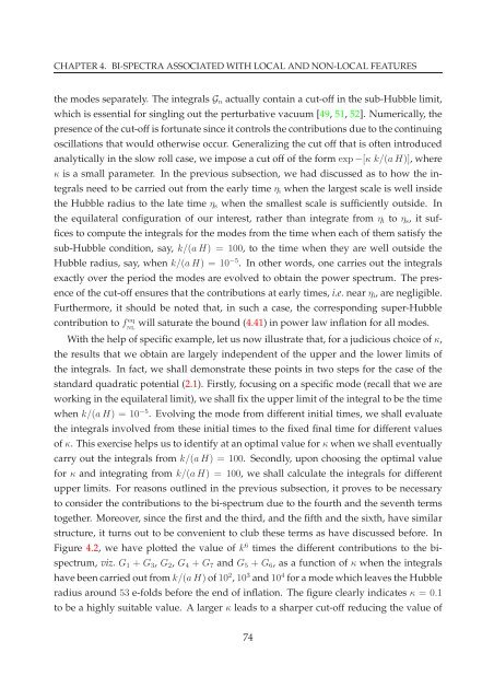
structure, it turns out to be convenient to club these terms as have discussed before. In
Figure 4.2, we have plotted the value of k 6 times the different contributions to the bispectrum,
viz. G 1 + G 3 , G 2 , G 4 + G 7 and G 5 + G 6 , as a function of κ when the integrals
have been carried out fromk/(aH) of10 2 ,10 3 and10 4 for a mode which leaves the Hubble
radius around 53 e-folds before the end of inflation. The figure clearly indicates κ = 0.1
to be a highly suitable value. A larger κ leads to a sharper cut-off reducing the value of
74