pdf-File - IAG - Universität Stuttgart

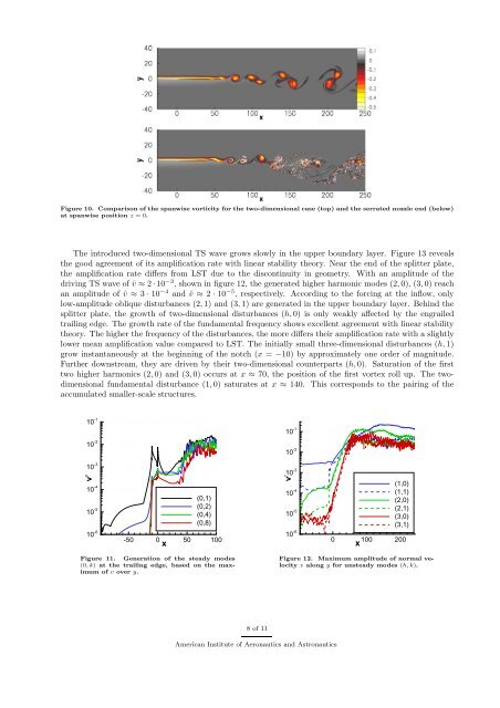
Figure 10. Comparison of the spanwise vorticity for the two-dimensional case (top) and the serrated nozzle end (below)
at spanwise position z = 0.
The introduced two-dimensional TS wave grows slowly in the upper boundary layer. Figure 13 reveals
the good agreement of its amplification rate with linear stability theory. Near the end of the splitter plate,
the amplification rate differs from LST due to the discontinuity in geometry. With an amplitude of the
driving TS wave of ˆv ≈ 2 · 10 −3 , shown in figure 12, the generated higher harmonic modes (2, 0), (3, 0) reach
an amplitude of ˆv ≈ 3 · 10 −4 and ˆv ≈ 2 · 10 −5 , respectively. According to the forcing at the inflow, only
low-amplitude oblique disturbances (2, 1) and (3, 1) are generated in the upper boundary layer. Behind the
splitter plate, the growth of two-dimensional disturbances (h, 0) is only weakly affected by the engrailed
trailing edge. The growth rate of the fundamental frequency shows excellent agreement with linear stability
theory. The higher the frequency of the disturbances, the more differs their amplification rate with a slightly
lower mean amplification value compared to LST. The initially small three-dimensional disturbances (h, 1)
grow instantaneously at the beginning of the notch (x = −10) by approximately one order of magnitude.
Further downstream, they are driven by their two-dimensional counterparts (h, 0). Saturation of the first
two higher harmonics (2, 0) and (3, 0) occurs at x ≈ 70, the position of the first vortex roll up. The twodimensional
fundamental disturbance (1, 0) saturates at x ≈ 140. This corresponds to the pairing of the
accumulated smaller-scale structures.
10 -2
10 -2
10 -3
v’
10 -1 (0,1)
10 -3
v’
10 -1 (1,0)
10 -4
10 -5
10 -6
-50 0 50 100
x
(0,2)
(0,4)
(0,8)
10 -4
10 -5
10 -6
0 100 200
x
(1,1)
(2,0)
(2,1)
(3,0)
(3,1)
Figure 11. Generation of the steady modes
(0, k) at the trailing edge, based on the maximum
of v over y.
Figure 12. Maximum amplitude of normal velocity
v along y for unsteady modes (h, k).
8 of 11
American Institute of Aeronautics and Astronautics