The Reduced Basis Method Problem Set 1

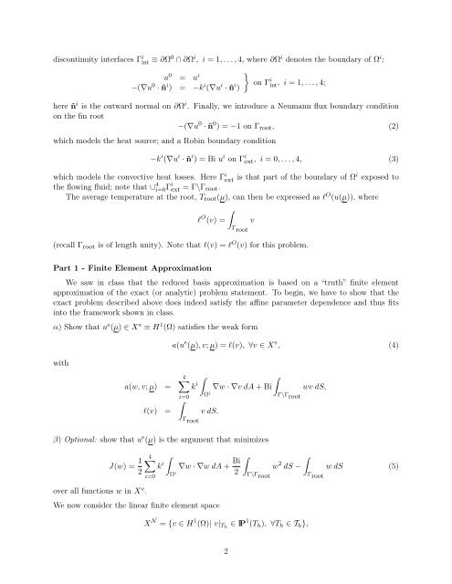
discontinuity interfaces Γ i int ≡ ∂Ω0 ∩ ∂Ω i , i = 1, . . . , 4, where ∂Ω i denotes the boundary of Ω i :
u 0 = u i
−(∇u 0 · ˆn i ) = −k i (∇u i · ˆn i )
}
on Γ i int, i = 1, . . . , 4;
here ˆn i is the outward normal on ∂Ω i . Finally, we introduce a Neumann flux boundary condition
on the fin root
−(∇u 0 · ˆn 0 ) = −1 on Γ root , (2)
which models the heat source; and a Robin boundary condition
−k i (∇u i · ˆn i ) = Bi u i on Γ i ext , i = 0, . . . , 4, (3)
which models the convective heat losses. Here Γ i ext is that part of the boundary of Ωi exposed to
the flowing fluid; note that ∪ 4 i=0Γ i ext = Γ\Γ root.
The average temperature at the root, T root (µ), can then be expressed as l O (u(µ)), where
∫
l O (v) = v
Γ root
(recall Γ root is of length unity). Note that l(v) = l O (v) for this problem.
Part 1 - Finite Element Approximation
We saw in class that the reduced basis approximation is based on a “truth” finite element
approximation of the exact (or analytic) problem statement. To begin, we have to show that the
exact problem described above does indeed satisfy the affine parameter dependence and thus fits
into the framework shown in class.
α) Show that u e (µ) ∈ X e ≡ H 1 (Ω) satisfies the weak form
a(u e (µ), v; µ) = l(v), ∀v ∈ X e , (4)
with
a(w, v; µ) =
l(v) =
4∑
∫
k i ∇w · ∇v dA + Bi wv dS,
i=0
∫Ω i Γ\Γ root
∫
v dS.
Γ root
β) Optional: show that u e (µ) is the argument that minimizes
J(w) = 1 2
4∑
∫
k i
i=0
∇w · ∇w dA + Bi
Ω i 2
∫
Γ\Γ root
∫
w 2 dS − w dS (5)
Γ root
over all functions w in X e .
We now consider the linear finite element space
X N = {v ∈ H 1 (Ω)| v| Th ∈ IP 1 (T h ), ∀T h ∈ T h },
2