The Reduced Basis Method Problem Set 1

Model Order Reduction Techniques I:
The Reduced Basis Method
Problem Set 1 – Linear Affine Elliptic Problems
Summer Term 2010, handed out 27.04.2010
Problem Statement – Design of a Thermal Fin
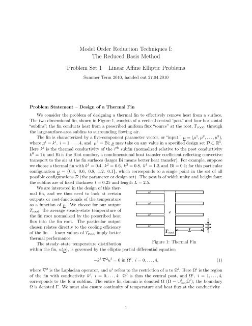
We consider the problem of designing a thermal fin to effectively remove heat from a surface.
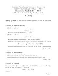
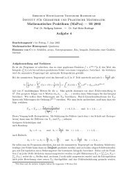
The two-dimensional fin, shown in Figure 1, consists of a vertical central “post” and four horizontal
“subfins”; the fin conducts heat from a prescribed uniform flux “source” at the root, Γ root , through
the large-surface-area subfins to surrounding flowing air.
The fin is characterized by a five-component parameter vector, or “input,” µ = (µ 1 , µ 2 , . . . , µ 5 ),
where µ i = k i , i = 1, . . . , 4, and µ 5 = Bi; µ may take on any value in a specified design set D ⊂ R 5 .
Here k i is the thermal conductivity of the i th subfin (normalized relative to the post conductivity
k 0 ≡ 1); and Bi is the Biot number, a nondimensional heat transfer coefficient reflecting convective
transport to the air at the fin surfaces (larger Bi means better heat transfer). For example, suppose
we choose a thermal fin with k 1 = 0.4, k 2 = 0.6, k 3 = 0.8, k 4 = 1.2, and Bi = 0.1; for this particular
configuration µ = {0.4, 0.6, 0.8, 1.2, 0.1}, which corresponds to a single point in the set of all
possible configurations D (the parameter or design set). The post is of width unity and height four;
the subfins are of fixed thickness t = 0.25 and length L = 2.5.
We are interested in the design of this thermal
fin, and we thus need to look at certain
outputs or cost-functionals of the temperature
as a function of µ. We choose for our output
T root , the average steady-state temperature of
the fin root normalized by the prescribed heat
flux into the fin root. The particular output
chosen relates directly to the cooling efficiency
of the fin — lower values of T root imply better
thermal performance.
The steady–state temperature distribution
Figure 1: Thermal Fin
within the fin, u(µ), is governed by the elliptic partial differential equation
−k i ∇ 2 u i = 0 in Ω i , i = 0, . . . , 4, (1)
where ∇ 2 is the Laplacian operator, and u i refers to the restriction of u to Ω i . Here Ω i is the region
of the fin with conductivity k i , i = 0, . . . , 4: Ω 0 is thus the central post, and Ω i , i = 1, . . . , 4,
corresponds to the four subfins. The entire fin domain is denoted Ω (¯Ω = ∪ 4 i=0 ¯Ω i ); the boundary
Ω is denoted Γ. We must also ensure continuity of temperature and heat flux at the conductivity–
1

discontinuity interfaces Γ i int ≡ ∂Ω0 ∩ ∂Ω i , i = 1, . . . , 4, where ∂Ω i denotes the boundary of Ω i :
u 0 = u i
−(∇u 0 · ˆn i ) = −k i (∇u i · ˆn i )
}
on Γ i int, i = 1, . . . , 4;
here ˆn i is the outward normal on ∂Ω i . Finally, we introduce a Neumann flux boundary condition
on the fin root
−(∇u 0 · ˆn 0 ) = −1 on Γ root , (2)
which models the heat source; and a Robin boundary condition
−k i (∇u i · ˆn i ) = Bi u i on Γ i ext , i = 0, . . . , 4, (3)
which models the convective heat losses. Here Γ i ext is that part of the boundary of Ωi exposed to
the flowing fluid; note that ∪ 4 i=0Γ i ext = Γ\Γ root.
The average temperature at the root, T root (µ), can then be expressed as l O (u(µ)), where
∫
l O (v) = v
Γ root
(recall Γ root is of length unity). Note that l(v) = l O (v) for this problem.
Part 1 - Finite Element Approximation
We saw in class that the reduced basis approximation is based on a “truth” finite element
approximation of the exact (or analytic) problem statement. To begin, we have to show that the
exact problem described above does indeed satisfy the affine parameter dependence and thus fits
into the framework shown in class.
α) Show that u e (µ) ∈ X e ≡ H 1 (Ω) satisfies the weak form
a(u e (µ), v; µ) = l(v), ∀v ∈ X e , (4)
with
a(w, v; µ) =
l(v) =
4∑
∫
k i ∇w · ∇v dA + Bi wv dS,
i=0
∫Ω i Γ\Γ root
∫
v dS.
Γ root
β) Optional: show that u e (µ) is the argument that minimizes
J(w) = 1 2
4∑
∫
k i
i=0
∇w · ∇w dA + Bi
Ω i 2
∫
Γ\Γ root
∫
w 2 dS − w dS (5)
Γ root
over all functions w in X e .
We now consider the linear finite element space
X N = {v ∈ H 1 (Ω)| v| Th ∈ IP 1 (T h ), ∀T h ∈ T h },
2

and look for u N (µ) ∈ X N such that
our output of interest is then given by
a(u N (µ), v; µ) = l(v), ∀v ∈ X N ; (6)
Applying our usual nodal basis, we arrive at the matrix equations
T N root (µ) = lO (u N (µ)). (7)
A N (µ) u N (µ) = F N ,
T N root (µ) = (LN ) T u N (µ),
where A N ∈ R N ×N , u N ∈ R N , F N ∈ R N , and L N ∈ R N ; here N is the dimension of the finite
element space X N , which (given our natural boundary conditions) is equal to the number of nodes
in T h .
Part 2 - Reduced-Basis Approximation
In general, the dimension of the finite element space, dim X = N , will be quite large (in
particular if we were to treat the more realistic three-dimensional fin problem), and thus the solution
of A N u N (µ) = F N can be quite expensive. We thus investigate the reduced-basis methods that allow
us to accurately and very rapidly predict T root (µ) in the limit of many evaluations — that is, at
many different values of µ — which is precisely the “limit of interest” in design and optimization
studies. To derive the reduced-basis approximation we shall exploit the energy principle,
u(µ) = arg min
w∈X J(w),
where J(w) is given by (5).
To begin, we introduce a sample in parameter space,
S N = {µ 1 , µ 2 , . . . , µ N }
with N ≪ N . Each µ i , i = 1, . . . , N, belongs in the parameter set D. For our parameter set we
choose D = [0.1, 10.0] 4 × [0.01, 1.0], that is, 0.1 ≤ k i ≤ 10.0, i = 1, . . . , 4, for the conductivities, and
0.01 ≤ Bi ≤ 1.0 for the Biot number.
We then introduce the reduced-basis space as
W N = span{u N (µ 1 ), u N (µ 2 ), . . . , u N (µ N )} (8)
where u N (µ i ) is the finite-element solution for µ = µ i . To simplify the notation, we define ζ i ∈ X
as
ζ i = u N (µ i ), i = 1, . . . , N;
we can then write W N = span{ζ i , i = 1, . . . , N}. Recall that W N = span{ζ i , i = 1, . . . , N} means
that W N consists of all functions in X that can be expressed as a linear combination of the ζ i ; that
is, any member v N of W N can be represented as
v N =
N∑
β j ζ j , (9)
j=1
3

for some unique choice of β j ∈ R, j = 1, . . . , N. (We implicitly assume that the ζ i , i = 1, . . . , N,
are linearly independent; it follows that W N is an N-dimensional subspace of X N .)
In the reduced-basis approach we look for an approximation u N (µ) to u N (µ) (which for our
purposes here we presume is arbitrarily close to u e (µ)) in W N ; in particular, we express u N (µ) as
u N (µ) =
N∑
u j N ζj ; (10)
j=1
we denote by u N (µ) ∈ R N the coefficient vector (u 1 N , . . . , uN N )T . The premise — or hope — is that
we should be able to accurately represent the solution at some new point in parameter space, µ, as
an appropriate linear combination of solutions previously computed at a small number of points in
parameter space (the µ i , i = 1, . . . , N). But how do we find this appropriate linear combination?
And how good is it? And how do we compute our approximation efficiently?
The energy principle is crucial here (though more generally the weak form would suffice). To
wit, we apply the classical Rayleigh-Ritz procedure to define
u N (µ) = arg
min J(w N ); (11)
w N ∈W N
alternatively we can apply Galerkin projection to obtain the equivalent statement
The output can then be calculated from
We now study this approximation in more detail.
α) Prove that, in the energy norm || · || ≡ (a(·, ·; µ)) 1/2 ,
a(u N (µ), v; µ) = l(v), ∀v ∈ W N . (12)
T root N (µ) = l O (u N (µ)). (13)
||u(µ) − u N (µ)|| ≤ ||u(µ) − w N ||, ∀w N ∈ W N . (14)
This inequality indicates that out of all the possible choices of w N in the space W N , the reducedbasis
method defined above will choose the “best one” (in the energy norm). Equivalently, we can
say that even if we knew the solution u(µ), we would not be able to find a better approximation to
u(µ) in W N — in the energy norm — than u N (µ).
β) Prove that
T root (µ) − T root N (µ) = ||u(µ) − u N (µ)|| 2 . (15)
γ) Show that u N (µ) as defined in (10–12) satisfies a set of N × N linear equations,
A N (µ)u N (µ) = F N ;
and that
T root N (µ) = L T N u N (µ).
Give expressions for A N (µ) ∈ R N×N in terms of A N (µ) and Z, F N ∈ R N in terms of F N and Z,
and L N ∈ R N in terms of L N and Z; here Z is an N × N matrix, the j th column of which is u N (µ j )
(the nodal values of u N (µ j )).
4

δ) Show that the bilinear form a(w, v; µ) can be decomposed as
a(w, v; µ) =
Q∑
Θ q (µ)a q (w, v), ∀w, v ∈ X, ∀µ ∈ D, (16)
q=1
for Q = 6; and give expressions for the Θ q (µ) and the a q (w, v). Notice that the a q (w, v) are not
dependent on µ; the parameter dependence enters only through the functions Θ q (µ), q = 1, . . . , Q.
Further show that
Q∑
A N (µ) = Θ q (µ)A N q ,
and
A N (µ) =
q=1
Q∑
Θ q (µ)A q N . (17)
q=1
Give an expression for the A N q in terms of the nodal basis functions; and develop a formula for the
A q N in terms of the AN q and Z.
Acknowledgment: This problem set is heavily based on a problem set in the class “16.920 Numerical
Methods for Partial Differential Equations” at MIT. Thanks to Prof. A.T. Patera and Debbie
Blanchard for providing the necessary material and for allowing us to use it.
5