Chapter 7 Rational Functions - College of the Redwoods
Chapter 7 Rational Functions - College of the Redwoods
Chapter 7 Rational Functions - College of the Redwoods

You also want an ePaper? Increase the reach of your titles
YUMPU automatically turns print PDFs into web optimized ePapers that Google loves.
7 <strong>Rational</strong> <strong>Functions</strong><br />
In this chapter, we begin our study <strong>of</strong> rational functions — functions <strong>of</strong> <strong>the</strong> form<br />
p(x)/q(x), where p and q are both polynomials. <strong>Rational</strong> functions are similar in<br />
structure to rational numbers (commonly thought <strong>of</strong> as fractions), and <strong>the</strong>y are studied<br />
and used extensively in ma<strong>the</strong>matics, engineering, and science.<br />
We will learn how to manipulate <strong>the</strong>se functions, and discover <strong>the</strong> myriad algebraic<br />
tricks and pitfalls that accompany <strong>the</strong>m. We will also see some <strong>of</strong> <strong>the</strong> ways that <strong>the</strong>y<br />
can be applied to everyday situations, such as modeling <strong>the</strong> length <strong>of</strong> time it takes a<br />
group <strong>of</strong> people to complete a task, or calculating <strong>the</strong> distance traveled by an object.<br />
In more advanced ma<strong>the</strong>matics courses, such as college algebra and calculus, you<br />
will learn even more about <strong>the</strong> intricate nature <strong>of</strong> rational functions. In many science<br />
and engineering courses, you will use rational functions to model what you are studying.<br />
In your everyday life, you can use rational functions for a number <strong>of</strong> useful calculations,<br />
such as <strong>the</strong> amount <strong>of</strong> time or work that a given task might require. For <strong>the</strong>se reasons,<br />
along with <strong>the</strong> fact that learning how to manipulate rational functions will fur<strong>the</strong>r your<br />
understanding <strong>of</strong> ma<strong>the</strong>matics, this chapter warrants a good deal <strong>of</strong> attention.<br />
Table <strong>of</strong> Contents<br />
7.1 Introducing <strong>Rational</strong> <strong>Functions</strong> . . . . . . . . . . . . . . . . . . . . . . . . . . . . . . . . . . . . 603<br />
The Graph <strong>of</strong> y = 1/x 604<br />
Translations 608<br />
Scaling and Reflection 609<br />
Difficulties with <strong>the</strong> Graphing Calculator 611<br />
Exercises 615<br />
Answers 617<br />
7.2 Reducing <strong>Rational</strong> <strong>Functions</strong> . . . . . . . . . . . . . . . . . . . . . . . . . . . . . . . . . . . . . . 619<br />
Cancellation 621<br />
Reducing <strong>Rational</strong> Expressions in x 623<br />
Sign Changes 627<br />
The Secant Line 630<br />
Exercises 633<br />
Answers 636<br />
7.3 Graphing <strong>Rational</strong> <strong>Functions</strong> . . . . . . . . . . . . . . . . . . . . . . . . . . . . . . . . . . . . . . 639<br />
The Domain <strong>of</strong> a <strong>Rational</strong> Function 639<br />
The Zeros <strong>of</strong> a <strong>Rational</strong> Function 643<br />
Drawing <strong>the</strong> Graph <strong>of</strong> a <strong>Rational</strong> Function 645<br />
Exercises 655<br />
Answers 657<br />
7.4 Products and Quotients <strong>of</strong> <strong>Rational</strong> <strong>Functions</strong> . . . . . . . . . . . . . . . . . . . . . . . 661<br />
Division <strong>of</strong> <strong>Rational</strong> Expressions 666<br />
Exercises 671<br />
Answers 676<br />
7.5 Sums and Differences <strong>of</strong> <strong>Rational</strong> <strong>Functions</strong> . . . . . . . . . . . . . . . . . . . . . . . . . 679<br />
601
602 <strong>Chapter</strong> 7 <strong>Rational</strong> <strong>Functions</strong><br />
Addition and Subtraction Defined 681<br />
Equivalent Fractions 683<br />
Adding and Subtracting Fractions with Different Denominators 683<br />
Exercises 691<br />
Answers 693<br />
7.6 Complex Fractions . . . . . . . . . . . . . . . . . . . . . . . . . . . . . . . . . . . . . . . . . . . . . . . 695<br />
Exercises 703<br />
Answers 708<br />
7.7 Solving <strong>Rational</strong> Equations . . . . . . . . . . . . . . . . . . . . . . . . . . . . . . . . . . . . . . . . 711<br />
Exercises 723<br />
Answers 727<br />
7.8 Applications <strong>of</strong> <strong>Rational</strong> <strong>Functions</strong> . . . . . . . . . . . . . . . . . . . . . . . . . . . . . . . . . 731<br />
Number Problems 731<br />
Distance, Speed, and Time Problems 734<br />
Work Problems 738<br />
Exercises 743<br />
Answers 746<br />
7.9 Index . . . . . . . . . . . . . . . . . . . . . . . . . . . . . . . . . . . . . . . . . . . . . . . . . . . . . . . . . . . 747<br />
Copyright<br />
All parts <strong>of</strong> this intermediate algebra textbook are copyrighted in <strong>the</strong> name <strong>of</strong><br />
Department <strong>of</strong> Ma<strong>the</strong>matics, <strong>College</strong> <strong>of</strong> <strong>the</strong> <strong>Redwoods</strong>. They are not in <strong>the</strong> public<br />
domain. However, <strong>the</strong>y are being made available free for use in educational institutions.<br />
This <strong>of</strong>fer does not extend to any application that is made for pr<strong>of</strong>it.<br />
Users who have such applications in mind should contact David Arnold at davidarnold@redwoods.edu<br />
or Bruce Wagner at bruce-wagner@redwoods.edu.<br />
This work (including all text, Portable Document Format files, and any o<strong>the</strong>r original<br />
works), except where o<strong>the</strong>rwise noted, is licensed under a Creative Commons<br />
Attribution-NonCommercial-ShareAlike 2.5 License, and is copyrighted C○2006,<br />
Department <strong>of</strong> Ma<strong>the</strong>matics, <strong>College</strong> <strong>of</strong> <strong>the</strong> <strong>Redwoods</strong>. To view a copy <strong>of</strong> this<br />
license, visit http://creativecommons.org/licenses/by-nc-sa/2.5/ or send a letter<br />
to Creative Commons, 543 Howard Street, 5th Floor, San Francisco, California,<br />
94105, USA.<br />
Version: Fall 2007
Section 7.1 Introducing <strong>Rational</strong> <strong>Functions</strong> 603<br />
7.1 Introducing <strong>Rational</strong> <strong>Functions</strong><br />
In <strong>the</strong> previous chapter, we studied polynomials, functions having equation form<br />
p(x) = a 0 + a 1 x + a 2 x 2 + · · · + a n x n . (1)<br />
Even though this polynomial is presented in ascending powers <strong>of</strong> x, <strong>the</strong> leading term<br />
<strong>of</strong> <strong>the</strong> polynomial is still a n x n , <strong>the</strong> term with <strong>the</strong> highest power <strong>of</strong> x. The degree <strong>of</strong><br />
<strong>the</strong> polynomial is <strong>the</strong> highest power <strong>of</strong> x present, so in this case, <strong>the</strong> degree <strong>of</strong> <strong>the</strong><br />
polynomial is n.<br />
In this section, our study will lead us to <strong>the</strong> rational functions. Note <strong>the</strong> root word<br />
“ratio” in <strong>the</strong> term “rational.” Does it remind you <strong>of</strong> <strong>the</strong> word “fraction”? It should,<br />
as rational functions are functions in a very specific fractional form.<br />
Definition 2. A rational function is a function that can be written as a quotient<br />
<strong>of</strong> two polynomial functions. In symbols, <strong>the</strong> function<br />
is called a rational function.<br />
f(x) = a 0 + a 1 x + a 2 x 2 + · · · + a n x n<br />
b 0 + b 1 x + b 2 x 2 + · · · + b m x m (3)<br />
For example,<br />
f(x) = 1 + x<br />
x + 2 , g(x) = x2 − 2x − 3<br />
, and h(x) =<br />
x + 4<br />
are rational functions, while<br />
3 − 2x − x 2<br />
x 3 + 2x 2 − 3x − 5<br />
(4)<br />
f(x) = 1 + √ x<br />
x 2 + 1 , g(x) = x2 + 2x − 3<br />
1 + x 1/2 − 3x 2 , and h(x) = √<br />
x 2 − 2x − 3<br />
x 2 + 4x − 12<br />
are not rational functions.<br />
Each <strong>of</strong> <strong>the</strong> functions in equation (4) are rational functions, because in each case,<br />
<strong>the</strong> numerator and denominator <strong>of</strong> <strong>the</strong> given expression is a valid polynomial.<br />
However, in equation (5), <strong>the</strong> numerator <strong>of</strong> f(x) is not a polynomial (polynomials<br />
do not allow <strong>the</strong> square root <strong>of</strong> <strong>the</strong> independent variable). Therefore, f is not a rational<br />
function.<br />
Similarly, <strong>the</strong> denominator <strong>of</strong> g(x) in equation (5) is not a polynomial. Fractions<br />
are not allowed as exponents in polynomials. Thus, g is not a rational function.<br />
Finally, in <strong>the</strong> case <strong>of</strong> function h in equation (5), although <strong>the</strong> radicand (<strong>the</strong><br />
expression inside <strong>the</strong> radical) is a rational function, <strong>the</strong> square root prevents h from<br />
being a rational function.<br />
(5)<br />
1<br />
Copyrighted material. See: http://msenux.redwoods.edu/IntAlgText/<br />
Version: Fall 2007
604 <strong>Chapter</strong> 7 <strong>Rational</strong> <strong>Functions</strong><br />
An important skill to develop is <strong>the</strong> ability to draw <strong>the</strong> graph <strong>of</strong> a rational function.<br />
Let’s begin by drawing <strong>the</strong> graph <strong>of</strong> one <strong>of</strong> <strong>the</strong> simplest (but most fundamental) rational<br />
functions.<br />
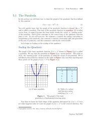
The Graph <strong>of</strong> y = 1/x<br />
In all new situations, when we are presented with an equation whose graph we’ve not<br />
considered or do not recognize, we begin <strong>the</strong> process <strong>of</strong> drawing <strong>the</strong> graph by creating<br />
a table <strong>of</strong> points that satisfy <strong>the</strong> equation. It’s important to remember that <strong>the</strong> graph<br />
<strong>of</strong> an equation is <strong>the</strong> set <strong>of</strong> all points that satisfy <strong>the</strong> equation. We note that zero is<br />
not in <strong>the</strong> domain <strong>of</strong> y = 1/x (division by zero makes no sense and is not defined), and<br />
create a table <strong>of</strong> points satisfying <strong>the</strong> equation shown in Figure 1.<br />
y<br />
10<br />
x<br />
10<br />
x y = 1/x<br />
−3 −1/3<br />
−2 −1/2<br />
−1<br />
−1<br />
1 1<br />
2 1/2<br />
3 1/3<br />
Figure 1. At <strong>the</strong> right is a table <strong>of</strong> points satisfying <strong>the</strong> equation y =<br />
1/x. These points are plotted as solid dots on <strong>the</strong> graph at <strong>the</strong> left.<br />
At this point (see Figure 1), it’s pretty clear what <strong>the</strong> graph is doing between<br />
x = −3 and x = −1. Likewise, it’s clear what is happening between x = 1 and x = 3.<br />
However, <strong>the</strong>re are some open areas <strong>of</strong> concern.<br />
1. What happens to <strong>the</strong> graph as x increases without bound? That is, what happens<br />
to <strong>the</strong> graph as x moves toward ∞?<br />
2. What happens to <strong>the</strong> graph as x decreases without bound? That is, what happens<br />
to <strong>the</strong> graph as x moves toward −∞?<br />
3. What happens to <strong>the</strong> graph as x approaches zero from <strong>the</strong> right?<br />
4. What happens to <strong>the</strong> graph as x approaches zero from <strong>the</strong> left?<br />
Let’s answer each <strong>of</strong> <strong>the</strong>se questions in turn. We’ll begin by discussing <strong>the</strong> “endbehavior”<br />
<strong>of</strong> <strong>the</strong> rational function defined by y = 1/x. First, <strong>the</strong> right end. What<br />
happens as x increases without bound? That is, what happens as x increases toward<br />
∞? In Table 1(a), we computed y = 1/x for x equalling 100, 1 000, and 10 000. Note<br />
how <strong>the</strong> y-values in Table 1(a) are all positive and approach zero.<br />
Students in calculus use <strong>the</strong> following notation for this idea.<br />
lim<br />
x→∞ y = lim<br />
x→∞<br />
1<br />
x = 0 (6)<br />
Version: Fall 2007
Section 7.1 Introducing <strong>Rational</strong> <strong>Functions</strong> 605<br />
They say “<strong>the</strong> limit <strong>of</strong> y as x approaches infinity is zero.” That is, as x approaches<br />
infinity, y approaches zero.<br />
x y = 1/x<br />
100 0.01<br />
1 000 0.001<br />
10 000 0.0001<br />
Table 1.<br />
(a)<br />
x y = 1/x<br />
−100 −0.01<br />
−1 000 −0.001<br />
−10 000 −0.0001<br />
(b)<br />
Examining <strong>the</strong> end-behavior <strong>of</strong> y = 1/x.<br />
A completely similar event happens at <strong>the</strong> left end. As x decreases without bound,<br />
that is, as x decreases toward −∞, note that <strong>the</strong> y-values in Table 1(b) are all negative<br />
and approach zero. Calculus students have a similar notation for this idea.<br />
lim y = lim 1<br />
= 0. (7)<br />
x→−∞ x→−∞ x<br />
They say “<strong>the</strong> limit <strong>of</strong> y as x approaches negative infinity is zero.”<br />
approaches negative infinity, y approaches zero.<br />
That is, as x<br />
These numbers in Tables 1(a) and 1(b), and <strong>the</strong> ideas described above, predict <strong>the</strong><br />
correct end-behavior <strong>of</strong> <strong>the</strong> graph <strong>of</strong> y = 1/x. At each end <strong>of</strong> <strong>the</strong> x-axis, <strong>the</strong> y-values<br />
must approach zero. This means that <strong>the</strong> graph <strong>of</strong> y = 1/x must approach <strong>the</strong> x-axis<br />
for x-values at <strong>the</strong> far right- and left-ends <strong>of</strong> <strong>the</strong> graph. In this case, we say that <strong>the</strong><br />
x-axis acts as a horizontal asymptote for <strong>the</strong> graph <strong>of</strong> y = 1/x. As x approaches ei<strong>the</strong>r<br />
positive or negative infinity, <strong>the</strong> graph <strong>of</strong> y = 1/x approaches <strong>the</strong> x-axis. This behavior<br />
is shown in Figure 2.<br />
y<br />
10<br />
x<br />
10<br />
Figure 2. The graph <strong>of</strong> 1/x approaches<br />
<strong>the</strong> x-axis as x increases or<br />
decreases without bound.<br />
Our last investigation will be on <strong>the</strong> interval from x = −1 to x = 1. Readers are<br />
again reminded that <strong>the</strong> function y = 1/x is undefined at x = 0. Consequently, we will<br />
break this region in half, first investigating what happens on <strong>the</strong> region between x = 0<br />
Version: Fall 2007
606 <strong>Chapter</strong> 7 <strong>Rational</strong> <strong>Functions</strong><br />
and x = 1. We evaluate y = 1/x at x = 1/2, x = 1/4, and x = 1/8, as shown in <strong>the</strong><br />
table in Figure 3, <strong>the</strong>n plot <strong>the</strong> resulting points.<br />
y<br />
10<br />
x<br />
10<br />
x y = 1/x<br />
1/2 2<br />
1/4 4<br />
1/8 8<br />
Figure 3. At <strong>the</strong> right is a table <strong>of</strong> points satisfying <strong>the</strong> equation y =<br />
1/x. These points are plotted as solid dots on <strong>the</strong> graph at <strong>the</strong> left.<br />
Note that <strong>the</strong> x-values in <strong>the</strong> table in Figure 3 approach zero from <strong>the</strong> right, <strong>the</strong>n<br />
note that <strong>the</strong> corresponding y-values are getting larger and larger. We could continue<br />
in this vein, adding points. For example, if x = 1/16, <strong>the</strong>n y = 16. If x = 1/32, <strong>the</strong>n<br />
y = 32. If x = 1/64, <strong>the</strong>n y = 64. Each time we halve our value <strong>of</strong> x, <strong>the</strong> resulting<br />
value <strong>of</strong> x is closer to zero, and <strong>the</strong> corresponding y-value doubles in size. Calculus<br />
students describe this behavior with <strong>the</strong> notation<br />
lim y = lim 1<br />
= ∞. (8)<br />
x→0 + x→0 + x<br />
That is, as “x approaches zero from <strong>the</strong> right, <strong>the</strong> value <strong>of</strong> y grows to infinity.” This is<br />
evident in <strong>the</strong> graph in Figure 3, where we see <strong>the</strong> plotted points move closer to <strong>the</strong><br />
vertical axis while at <strong>the</strong> same time moving upward without bound.<br />
A similar thing happens on <strong>the</strong> o<strong>the</strong>r side <strong>of</strong> <strong>the</strong> vertical axis, as shown in Figure 4.<br />
y<br />
10<br />
x<br />
10<br />
x y = 1/x<br />
−1/2 −2<br />
−1/4 −4<br />
−1/8 −8<br />
Figure 4. At <strong>the</strong> right is a table <strong>of</strong> points satisfying <strong>the</strong> equation y =<br />
1/x. These points are plotted as solid dots on <strong>the</strong> graph at <strong>the</strong> left.<br />
Version: Fall 2007
Section 7.1 Introducing <strong>Rational</strong> <strong>Functions</strong> 607<br />
Again, calculus students would write<br />
lim y = lim 1<br />
= −∞. (9)<br />
x→0 − x→0 − x<br />
That is, “as x approaches zero from <strong>the</strong> left, <strong>the</strong> values <strong>of</strong> y decrease to negative infinity.”<br />
In Figure 4, it is clear that as points move closer to <strong>the</strong> vertical axis (as x approaches<br />
zero) from <strong>the</strong> left, <strong>the</strong> graph decreases without bound.<br />
The evidence ga<strong>the</strong>red to this point indicates that <strong>the</strong> vertical axis is acting as a<br />
vertical asymptote. As x approaches zero from ei<strong>the</strong>r side, <strong>the</strong> graph approaches <strong>the</strong><br />
vertical axis, ei<strong>the</strong>r rising to infinity, or falling to negative infinity. The graph cannot<br />
cross <strong>the</strong> vertical axis because <strong>the</strong> function is undefined <strong>the</strong>re. The completed graph is<br />
shown in Figure 5.<br />
y<br />
10<br />
x<br />
10<br />
Figure 5. The completed graph <strong>of</strong><br />
y = 1/x. Note how <strong>the</strong> x-axis acts as a<br />
horizontal asymptote, while <strong>the</strong> y-axis<br />
acts as a vertical asymptote.<br />
The complete graph <strong>of</strong> y = 1/x in Figure 5 is called a hyperbola and serves as a<br />
fundamental starting point for all subsequent discussion in this section.<br />
We noted earlier that <strong>the</strong> domain <strong>of</strong> <strong>the</strong> function defined by <strong>the</strong> equation y = 1/x is<br />
<strong>the</strong> set D = {x : x ≠ 0}. Zero is excluded from <strong>the</strong> domain because division by zero is<br />
undefined. It’s no coincidence that <strong>the</strong> graph has a vertical asymptote at x = 0. We’ll<br />
see this relationship reinforced in fur<strong>the</strong>r examples.<br />
Version: Fall 2007
608 <strong>Chapter</strong> 7 <strong>Rational</strong> <strong>Functions</strong><br />
Translations<br />
In this section, we will translate <strong>the</strong> graph <strong>of</strong> y = 1/x in both <strong>the</strong> horizontal and vertical<br />
directions.<br />
◮ Example 10.<br />
Sketch <strong>the</strong> graph <strong>of</strong><br />
y = 1 − 4. (11)<br />
x + 3<br />
Technically, <strong>the</strong> function defined by y = 1/(x + 3) − 4 does not have <strong>the</strong> general<br />
form (3) <strong>of</strong> a rational function. However, in later chapters we will show how y =<br />
1/(x + 3) − 4 can be manipulated into <strong>the</strong> general form <strong>of</strong> a rational function.<br />
We know what <strong>the</strong> graph <strong>of</strong> y = 1/x looks like. If we replace x with x + 3, this will<br />
shift <strong>the</strong> graph <strong>of</strong> y = 1/x three units to <strong>the</strong> left, as shown in Figure 6(a). Note that<br />
<strong>the</strong> vertical asymptote has also shifted 3 units to <strong>the</strong> left <strong>of</strong> its original position (<strong>the</strong><br />
y-axis) and now has equation x = −3. By tradition, we draw <strong>the</strong> vertical asymptote<br />
as a dashed line.<br />
If we subtract 4 from <strong>the</strong> result in Figure 6(a), this will shift <strong>the</strong> graph in Figure 6(a)<br />
four units downward to produce <strong>the</strong> graph shown in Figure 6(b). Note that <strong>the</strong> horizontal<br />
asymptote also shifted 4 units downward from its original position (<strong>the</strong> x-axis)<br />
and now has equation y = −4.<br />
x = −3<br />
y<br />
10<br />
x = −3<br />
y<br />
10<br />
x<br />
10<br />
x<br />
10<br />
y = −4<br />
(a) y = 1/(x + 3) (b) y = 1/(x + 3) − 4<br />
Figure 6. Shifting <strong>the</strong> graph <strong>of</strong> y = 1/x.<br />
If you examine equation (11), you note that you cannot use x = −3 as this will<br />
make <strong>the</strong> denominator <strong>of</strong> equation (11) equal to zero. In Figure 6(b), note that<br />
<strong>the</strong>re is a vertical asymptote in <strong>the</strong> graph <strong>of</strong> equation (11) at x = −3. This is a<br />
common occurrence, which will be a central <strong>the</strong>me <strong>of</strong> this chapter.<br />
Version: Fall 2007
Section 7.1 Introducing <strong>Rational</strong> <strong>Functions</strong> 609<br />
Let’s ask ano<strong>the</strong>r key question.<br />
◮ Example 12.<br />
in Example 10?<br />
You can glance at <strong>the</strong> equation<br />
What are <strong>the</strong> domain and range <strong>of</strong> <strong>the</strong> rational function presented<br />
y = 1<br />
x + 3 − 4<br />
<strong>of</strong> Example 10 and note that x = −3 makes <strong>the</strong> denominator zero and must be<br />
excluded from <strong>the</strong> domain. Hence, <strong>the</strong> domain <strong>of</strong> this function is D = {x : x ≠ −3}.<br />
However, you can also determine <strong>the</strong> domain by examining <strong>the</strong> graph <strong>of</strong> <strong>the</strong> function<br />
in Figure 6(b). Note that <strong>the</strong> graph extends indefinitely to <strong>the</strong> left and right. One<br />
might first guess that <strong>the</strong> domain is all real numbers if it were not for <strong>the</strong> vertical<br />
asymptote at x = −3 interrupting <strong>the</strong> continuity <strong>of</strong> <strong>the</strong> graph. Because <strong>the</strong> graph <strong>of</strong><br />
<strong>the</strong> function gets arbitrarily close to this vertical asymptote (on ei<strong>the</strong>r side) without<br />
actually touching <strong>the</strong> asymptote, <strong>the</strong> graph does not contain a point having an x-value<br />
equaling −3. Hence, <strong>the</strong> domain is as above, D = {x : x ≠ −3}. This is comforting that<br />
<strong>the</strong> graphical analysis agrees with our earlier analytical determination <strong>of</strong> <strong>the</strong> domain.<br />
The graph is especially helpful in determining <strong>the</strong> range <strong>of</strong> <strong>the</strong> function. Note that<br />
<strong>the</strong> graph rises to positive infinity and falls to negative infinity. One would first guess<br />
that <strong>the</strong> range is all real numbers if it were not for <strong>the</strong> horizontal asymptote at y = −4<br />
interrupting <strong>the</strong> continuity <strong>of</strong> <strong>the</strong> graph. Because <strong>the</strong> graph gets arbitrarily close to<br />
<strong>the</strong> horizontal asymptote (on ei<strong>the</strong>r side) without actually touching <strong>the</strong> asymptote, <strong>the</strong><br />
graph does not contain a point having a y-value equaling −4. Hence, −4 is excluded<br />
from <strong>the</strong> range. That is, R = {y : y ≠ −4}.<br />
Scaling and Reflection<br />
In this section, we will both scale and reflect <strong>the</strong> graph <strong>of</strong> y = 1/x. For extra measure,<br />
we also throw in translations in <strong>the</strong> horizontal and vertical directions.<br />
◮ Example 13.<br />
Sketch <strong>the</strong> graph <strong>of</strong><br />
First, we multiply <strong>the</strong> equation y = 1/x by −2 to get<br />
y = − 2 + 3. (14)<br />
x − 4<br />
y = − 2 x .<br />
Multiplying by 2 should stretch <strong>the</strong> graph in <strong>the</strong> vertical directions (both positive and<br />
negative) by a factor <strong>of</strong> 2. Note that points that are very near <strong>the</strong> x-axis, when doubled,<br />
are not going to stray too far from <strong>the</strong> x-axis, so <strong>the</strong> horizontal asymptote will remain<br />
<strong>the</strong> same. Finally, multiplying by −2 will not only stretch <strong>the</strong> graph, it will also reflect<br />
<strong>the</strong> graph across <strong>the</strong> x-axis, as shown in Figure 7(b). 2<br />
2 Recall that we saw similar behavior when studying <strong>the</strong> parabola. The graph <strong>of</strong> y = −2x 2 stretched<br />
(vertically) <strong>the</strong> graph <strong>of</strong> <strong>the</strong> equation y = x 2 by a factor <strong>of</strong> 2, <strong>the</strong>n reflected <strong>the</strong> result across <strong>the</strong> x-axis.<br />
Version: Fall 2007
610 <strong>Chapter</strong> 7 <strong>Rational</strong> <strong>Functions</strong><br />
y<br />
10<br />
y<br />
10<br />
x<br />
10<br />
x<br />
10<br />
(a) y = 1/x<br />
Figure 7.<br />
(b) y = −2/x<br />
Scaling and reflecting <strong>the</strong> graph <strong>of</strong> y = 1/x.<br />
Replacing x with x − 4 will shift <strong>the</strong> graph 4 units to <strong>the</strong> right, <strong>the</strong>n adding 3 will<br />
shift <strong>the</strong> graph 3 units up, as shown in Figure 8. Note again that x = 4 makes <strong>the</strong><br />
denominator <strong>of</strong> y = −2/(x − 4) + 3 equal to zero and <strong>the</strong>re is a vertical asymptote at<br />
x = 4. The domain <strong>of</strong> this function is D = {x : x ≠ 4}.<br />
As x approaches positive or negative infinity, points on <strong>the</strong> graph <strong>of</strong> y = −2/(x−4)+<br />
3 get arbitrarily close to <strong>the</strong> horizontal asymptote y = 3 but never touch it. Therefore,<br />
<strong>the</strong>re is no point on <strong>the</strong> graph that has a y-value <strong>of</strong> 3. Thus, <strong>the</strong> range <strong>of</strong> <strong>the</strong> function<br />
is <strong>the</strong> set R = {y : y ≠ 3}.<br />
y<br />
10 x = 4<br />
y = 3<br />
x<br />
10<br />
Figure 8. The graph <strong>of</strong> y = −2/(x −<br />
4) + 3 is shifted 4 units right and 3 units<br />
up.<br />
Version: Fall 2007
Section 7.1 Introducing <strong>Rational</strong> <strong>Functions</strong> 611<br />
Difficulties with <strong>the</strong> Graphing Calculator<br />
The graphing calculator does a very good job drawing <strong>the</strong> graphs <strong>of</strong> “continuous functions.”<br />
A continuous function is one that can be drawn in one continuous stroke, never<br />
lifting pen or pencil from <strong>the</strong> paper during <strong>the</strong> drawing.<br />
Polynomials, such as <strong>the</strong> one in Figure 9, are continuous functions.<br />
y<br />
50<br />
x<br />
10<br />
Figure 9. A polynomial is a continuous<br />
function.<br />
Unfortunately, a rational function with vertical asymptote(s) is not a continuous function.<br />
First, you have to lift your pen at points where <strong>the</strong> denominator is zero, because<br />
<strong>the</strong> function is undefined at <strong>the</strong>se points. Secondly, it’s not uncommon to have to<br />
jump from positive infinity to negative infinity (or vice-versa) when crossing a vertical<br />
asymptote. When this happens, we have to lift our pen and shift it before continuing<br />
with our drawing.<br />
However, <strong>the</strong> graphing calculator does not know how to do this “lifting” <strong>of</strong> <strong>the</strong> pen<br />
near vertical asymptotes. The graphing calculator only knows one technique, plot a<br />
point, <strong>the</strong>n connect it with a segment to <strong>the</strong> last point plotted, move an incremental<br />
distance and repeat. Consequently, when <strong>the</strong> graphing calculator crosses a vertical<br />
asymptote where <strong>the</strong>re is a shift from one type <strong>of</strong> infinity to ano<strong>the</strong>r (e.g., from positive<br />
to negative), <strong>the</strong> calculator draws a “false line” <strong>of</strong> connection, one that it should not<br />
draw. Let’s demonstrate this aberration with an example.<br />
◮ Example 15.<br />
in Example 13.<br />
Use a graphing calculator to draw <strong>the</strong> graph <strong>of</strong> <strong>the</strong> rational function<br />
Load <strong>the</strong> equation into your calculator, as shown in Figure 10(a). Set <strong>the</strong> window<br />
as shown in Figure 10(b), <strong>the</strong>n push <strong>the</strong> GRAPH button to draw <strong>the</strong> graph shown in<br />
Figure 10(c). Results may differ on some calculators, but in our case, note <strong>the</strong> “false<br />
Version: Fall 2007
612 <strong>Chapter</strong> 7 <strong>Rational</strong> <strong>Functions</strong><br />
line” drawn from <strong>the</strong> top <strong>of</strong> <strong>the</strong> screen to <strong>the</strong> bottom, attempting to “connect” <strong>the</strong> two<br />
branches <strong>of</strong> <strong>the</strong> hyperbola.<br />
Some might rejoice and claim, “Hey, my graphing calculator draws vertical asymptotes.”<br />
However, before you get too excited, note that in Figure 8 <strong>the</strong> vertical<br />
asymptote should occur at exactly x = 4. If you look very carefully at <strong>the</strong> “vertical<br />
line” in Figure 10(c), you’ll note that it just misses <strong>the</strong> tick mark at x = 4. This “vertical<br />
line” is a line that <strong>the</strong> calculator should not draw. The calculator is attempting<br />
to draw a continuous function where one doesn’t exist.<br />
Figure 10.<br />
(a) (b) (c)<br />
The calculator attempts to draw a continuous function when it shouldn’t.<br />
One possible workaround 3 is to press <strong>the</strong> MODE button on your keyboard, which<br />
opens <strong>the</strong> menu shown in Figure 11(a). Use <strong>the</strong> arrow keys to highlight DOT instead<br />
<strong>of</strong> CONNECTED and press <strong>the</strong> ENTER key to make <strong>the</strong> selection permanent. Press <strong>the</strong><br />
GRAPH button to draw <strong>the</strong> graph in Figure 11(b).<br />
(a)<br />
Figure 11.<br />
(b)<br />
The same graph in “dot mode.”<br />
This “dot mode” on your calculator calculates <strong>the</strong> next point on <strong>the</strong> graph and plots<br />
<strong>the</strong> point, but it does not connect it with a line segment to <strong>the</strong> previously plotted<br />
point. This mode is useful in demonstrating that <strong>the</strong> vertical line in Figure 10(c) is<br />
not really part <strong>of</strong> <strong>the</strong> graph, but we lose some parts <strong>of</strong> <strong>the</strong> graph we’d really like to see.<br />
Compromise is in order.<br />
This example clearly shows that intelligent use <strong>of</strong> <strong>the</strong> calculator is a required component<br />
<strong>of</strong> this course. The calculator is not simply a “black box” that automatically<br />
does what you want it to do. In particular, when you are drawing rational functions,<br />
it helps to know ahead <strong>of</strong> time <strong>the</strong> placement <strong>of</strong> <strong>the</strong> vertical asymptotes. Knowledge<br />
3 Instructors might discuss a number <strong>of</strong> alternative strategies to represent rational functions on <strong>the</strong><br />
graphing calculator. What we present here is only one <strong>of</strong> a number <strong>of</strong> approaches.<br />
Version: Fall 2007
Section 7.1 Introducing <strong>Rational</strong> <strong>Functions</strong> 613<br />
<strong>of</strong> <strong>the</strong> asymptotes, coupled with what you see on your calculator screen, should enable<br />
you to draw a graph as accurate as that shown in Figure 8.<br />
Gentle reminder. You’ll want to set your calculator back in “connected mode.”<br />
To do this, press <strong>the</strong> MODE button on your keyboard to open <strong>the</strong> menu in Figure 10(a)<br />
once again. Use your arrow keys to highlight CONNECTED, <strong>the</strong>n press <strong>the</strong> ENTER key to<br />
make <strong>the</strong> selection permanent.<br />
Version: Fall 2007
614 <strong>Chapter</strong> 7 <strong>Rational</strong> <strong>Functions</strong><br />
Version: Fall 2007
Section 7.1 Introducing <strong>Rational</strong> <strong>Functions</strong> 615<br />
7.1 Exercises<br />
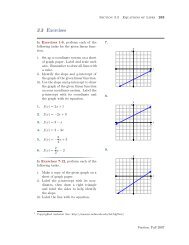
In Exercises 1-14, perform each <strong>of</strong> <strong>the</strong><br />
following tasks for <strong>the</strong> given rational function.<br />
i. Set up a coordinate system on a sheet<br />
<strong>of</strong> graph paper. Label and scale each<br />
axis.<br />
ii. Use geometric transformations as in<br />
Examples 10, 12, and 13 to draw <strong>the</strong><br />
graphs <strong>of</strong> each <strong>of</strong> <strong>the</strong> following rational<br />
functions. Draw <strong>the</strong> vertical<br />
and horizontal asymptotes as dashed<br />
lines and label each with its equation.<br />
You may use your calculator to<br />
check your solution, but you should<br />
be able to draw <strong>the</strong> rational function<br />
without <strong>the</strong> use <strong>of</strong> a calculator.<br />
iii. Use set-builder notation to describe<br />
<strong>the</strong> domain and range <strong>of</strong> <strong>the</strong> given<br />
rational function.<br />
1. f(x) = −2/x<br />
2. f(x) = 3/x<br />
3. f(x) = 1/(x − 4)<br />
4. f(x) = 1/(x + 3)<br />
5. f(x) = 2/(x − 5)<br />
6. f(x) = −3/(x + 6)<br />
7. f(x) = 1/x − 2<br />
8. f(x) = −1/x + 4<br />
9. f(x) = −2/x − 5<br />
10. f(x) = 3/x − 5<br />
11. f(x) = 1/(x − 2) − 3<br />
12. f(x) = −1/(x + 1) + 5<br />
13. f(x) = −2/(x − 3) − 4<br />
14. f(x) = 3/(x + 5) − 2<br />
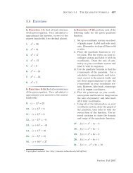
In Exercises 15-22, find all vertical asymptotes,<br />
if any, <strong>of</strong> <strong>the</strong> graph <strong>of</strong> <strong>the</strong> given<br />
function.<br />
15. f(x) = − 5<br />
x + 1 − 3<br />
16. f(x) = 6<br />
x + 8 + 2<br />
17. f(x) = − 9<br />
x + 2 − 6<br />
18. f(x) = − 8<br />
x − 4 − 5<br />
19. f(x) = 2<br />
x + 5 + 1<br />
20. f(x) = − 3<br />
x + 9 + 2<br />
21. f(x) = 7<br />
x + 8 − 9<br />
22. f(x) = 6<br />
x − 5 − 8<br />
In Exercises 23-30, find all horizontal<br />
asymptotes, if any, <strong>of</strong> <strong>the</strong> graph <strong>of</strong> <strong>the</strong><br />
given function.<br />
23. f(x) = 5<br />
x + 7 + 9<br />
24. f(x) = − 8<br />
x + 7 − 4<br />
4<br />
Copyrighted material. See: http://msenux.redwoods.edu/IntAlgText/<br />
Version: Fall 2007
616 <strong>Chapter</strong> 7 <strong>Rational</strong> <strong>Functions</strong><br />
25. f(x) = 8<br />
x + 5 − 1<br />
26. f(x) = − 2<br />
x + 3 + 8<br />
27. f(x) = 7<br />
x + 1 − 9<br />
28. f(x) = − 2<br />
x − 1 + 5<br />
29. f(x) = 5<br />
x + 2 − 4<br />
30. f(x) = − 6<br />
x − 1 − 2<br />
In Exercises 31-38, state <strong>the</strong> domain<br />
<strong>of</strong> <strong>the</strong> given rational function using setbuilder<br />
notation.<br />
31. f(x) = 4<br />
x + 5 + 5<br />
32. f(x) = − 7<br />
x − 6 + 1<br />
In Exercises 39-46, find <strong>the</strong> range <strong>of</strong><br />
<strong>the</strong> given function, and express your answer<br />
in set notation.<br />
39. f(x) = 2<br />
x − 3 + 8<br />
40. f(x) = 4<br />
x − 3 + 5<br />
41. f(x) = − 5<br />
x − 8 − 5<br />
42. f(x) = − 2<br />
x + 1 + 6<br />
43. f(x) = 7<br />
x + 7 + 5<br />
44. f(x) = − 8<br />
x + 3 + 9<br />
45. f(x) = 4<br />
x + 3 − 2<br />
46. f(x) = − 5<br />
x − 4 + 9<br />
33. f(x) = 6<br />
x − 5 + 1<br />
34. f(x) = − 5<br />
x − 3 − 9<br />
35. f(x) = 1<br />
x + 7 + 2<br />
36. f(x) = − 2<br />
x − 5 + 4<br />
37. f(x) = − 4<br />
x + 2 + 2<br />
38. f(x) = 2<br />
x + 6 + 9<br />
Version: Fall 2007
Section 7.1 Introducing <strong>Rational</strong> <strong>Functions</strong> 617<br />
7.1 Answers<br />
1. D = {x : x ≠ 0}, R = {y : y ≠ 0}<br />
y<br />
10<br />
7. D = {x : x ≠ 0}, R = {y : y ≠ −2}<br />
y<br />
10<br />
y=0<br />
x<br />
10<br />
y=−2<br />
x<br />
10<br />
x=0<br />
x=0<br />
3. D = {x : x ≠ 4}, R = {y : y ≠ 0}<br />
y<br />
10<br />
9. D = {x : x ≠ 0}, R = {y : y ≠ −5}<br />
y<br />
10<br />
y=0<br />
x<br />
10<br />
x<br />
10<br />
y=−5<br />
x=4<br />
x=0<br />
5. D = {x : x ≠ 5}, R = {y : y ≠ 0}<br />
y<br />
10<br />
11. D = {x : x ≠ 2}, R = {y : y ≠<br />
−3}<br />
y<br />
10<br />
y=0<br />
x<br />
10<br />
x<br />
10<br />
y=−3<br />
x=5<br />
x=2<br />
Version: Fall 2007
618 <strong>Chapter</strong> 7 <strong>Rational</strong> <strong>Functions</strong><br />
13. D = {x : x ≠ 3}, R = {y : y ≠<br />
−4}<br />
y<br />
10<br />
x=3<br />
y=−4<br />
x<br />
10<br />
15. Vertical asymptote: x = −1<br />
17. Vertical asymptote: x = −2<br />
19. Vertical asymptote: x = −5<br />
21. Vertical asymptote: x = −8<br />
23. Horizontal asymptote: y = 9<br />
25. Horizontal asymptote: y = −1<br />
27. Horizontal asymptote: y = −9<br />
29. Horizontal asymptote: y = −4<br />
31. Domain = {x : x ≠ −5}<br />
33. Domain = {x : x ≠ 5}<br />
35. Domain = {x : x ≠ −7}<br />
37. Domain = {x : x ≠ −2}<br />
39. Range = {y : y ≠ 8}<br />
41. Range = {y : y ≠ −5}<br />
43. Range = {y : y ≠ 5}<br />
45. Range = {y : y ≠ −2}<br />
Version: Fall 2007
Section 7.2 Reducing <strong>Rational</strong> <strong>Functions</strong> 619<br />
7.2 Reducing <strong>Rational</strong> <strong>Functions</strong><br />
The goal <strong>of</strong> this section is to learn how to reduce a rational expression to “lowest terms.”<br />
Of course, that means that we will have to understand what is meant by <strong>the</strong> phrase<br />
“lowest terms.” With that thought in mind, we begin with a discussion <strong>of</strong> <strong>the</strong> greatest<br />
common divisor <strong>of</strong> a pair <strong>of</strong> integers.<br />
First, we define what we mean by “divisibility.”<br />
Definition 1. Suppose that we have a pair <strong>of</strong> integers a and b. We say that “a<br />
is a divisor <strong>of</strong> b,” or “a divides b” if and only if <strong>the</strong>re is ano<strong>the</strong>r integer k so that<br />
b = ak. Ano<strong>the</strong>r way <strong>of</strong> saying <strong>the</strong> same thing is to say that a divides b if, upon<br />
dividing b by a, <strong>the</strong> remainder is zero.<br />
Let’s look at an example.<br />
◮ Example 2. What are <strong>the</strong> divisors <strong>of</strong> 12?<br />
Because 12 = 1 × 12, both 1 and 12 are divisors 6 <strong>of</strong> 12. Because 12 = 2 × 6, both 2<br />
and 6 are divisors <strong>of</strong> 12. Finally, because 12 = 3 × 4, both 3 and 4 are divisors <strong>of</strong> 12.<br />
If we list <strong>the</strong>m in ascending order, <strong>the</strong> divisors <strong>of</strong> 12 are<br />
1, 2, 3, 4, 6, and 12.<br />
Let’s look at ano<strong>the</strong>r example.<br />
◮ Example 3. What are <strong>the</strong> divisors <strong>of</strong> 18?<br />
Because 18 = 1 × 18, both 1 and 18 are divisors <strong>of</strong> 18. Similarly, 18 = 2 × 9 and<br />
18 = 3 × 6, so in ascending order, <strong>the</strong> divisors <strong>of</strong> 18 are<br />
1, 2, 3, 6, 9, and 18.<br />
The greatest common divisor <strong>of</strong> two or more integers is <strong>the</strong> largest divisor <strong>the</strong><br />
integers share in common. An example should make this clear.<br />
◮ Example 4. What is <strong>the</strong> greatest common divisor <strong>of</strong> 12 and 18?<br />
In Example 2 and Example 3, we saw <strong>the</strong> following.<br />
Divisors <strong>of</strong> 12 : 1 , 2 , 3 , 4, 6 , 12<br />
Divisors <strong>of</strong> 18 : 1 , 2 , 3 , 6 , 9, 18<br />
5<br />
Copyrighted material. See: http://msenux.redwoods.edu/IntAlgText/<br />
6 The word “divisor” and <strong>the</strong> word “factor” are synonymous.<br />
Version: Fall 2007
620 <strong>Chapter</strong> 7 <strong>Rational</strong> <strong>Functions</strong><br />
We’ve framed <strong>the</strong> divisors that 12 and 18 have in common. They are 1, 2, 3, and 6. The<br />
“greatest” <strong>of</strong> <strong>the</strong>se “common” divisors is 6. Hence, we say that “<strong>the</strong> greatest common<br />
divisor <strong>of</strong> 12 and 18 is 6.”<br />
Definition 5. The greatest common divisor <strong>of</strong> two integers a and b is <strong>the</strong> largest<br />
divisor <strong>the</strong>y have in common. We will use <strong>the</strong> notation<br />
GCD(a, b)<br />
to represent <strong>the</strong> greatest common divisor <strong>of</strong> a and b.<br />
Thus, as we saw in Example 4, GCD(12, 18) = 6.<br />
When <strong>the</strong> greatest common divisor <strong>of</strong> a pair <strong>of</strong> integers is one, we give that pair a<br />
special name.<br />
Definition 6. Let a and b be integers. If <strong>the</strong> greatest common divisor <strong>of</strong> a and<br />
b is one, that is, if GCD(a, b) = 1, <strong>the</strong>n we say that a and b are relatively prime.<br />
For example:<br />
• 9 and 12 are not relatively prime because GCD(9, 12) = 3.<br />
• 10 and 15 are not relatively prime because GCD(10, 15) = 5.<br />
• 8 and 21 are relatively prime because GCD(8, 21) = 1.<br />
We can now define what is meant when we say that a rational number is reduced<br />
to lowest terms.<br />
Definition 7. A rational number in <strong>the</strong> form p/q, where p and q are integers,<br />
is said to be reduced to lowest terms if and only if GCD(p, q) = 1. That is, p/q<br />
is reduced to lowest terms if <strong>the</strong> greatest common divisor <strong>of</strong> both numerator and<br />
denominator is 1.<br />
As we saw in Example 4, <strong>the</strong> greatest common divisor <strong>of</strong> 12 and 18 is 6. Therefore,<br />
<strong>the</strong> fraction 12/18 is not reduced to lowest terms. However, we can reduce 12/18 to<br />
lowest terms by dividing both numerator and denominator by <strong>the</strong>ir greatest common<br />
divisor. That is,<br />
12<br />
18 = 12 ÷ 6<br />
18 ÷ 6 = 2 3 .<br />
Note that GCD(2, 3) = 1, so 2/3 is reduced to lowest terms.<br />
Version: Fall 2007
Section 7.2 Reducing <strong>Rational</strong> <strong>Functions</strong> 621<br />
When it is difficult to ascertain <strong>the</strong> greatest common divisor, we’ll find it more<br />
efficient to proceed as follows:<br />
• Prime factor both numerator and denominator.<br />
• Cancel common factors.<br />
Thus, to reduce 12/18 to lowest terms, first express both numerator and denominator<br />
as a product <strong>of</strong> prime numbers, <strong>the</strong>n cancel common primes.<br />
12<br />
18 = 2 · 2 · 3<br />
2 · 3 · 3 = 2 · 2 · 3<br />
2 · 3 · 3 = 2 3<br />
When you cancel a 2, you’re actually dividing both numerator and denominator by 2.<br />
When you cancel a 3, you’re actually dividing both numerator and denominator by 3.<br />
Note that doing both (dividing by 2 and <strong>the</strong>n dividing by 3) is equivalent to dividing<br />
both numerator and denominator by 6.<br />
We will favor this latter technique, precisely because it is identical to <strong>the</strong> technique<br />
we will use to reduce rational functions to lowest terms. However, this “cancellation”<br />
technique has some pitfalls, so let’s take a moment to discuss some common cancellation<br />
mistakes.<br />
Cancellation<br />
You can spark some pretty heated debate amongst ma<strong>the</strong>matics educators by innocently<br />
mentioning <strong>the</strong> word “cancellation.” There seem to be two diametrically opposed camps,<br />
those who don’t mind when <strong>the</strong>ir students use <strong>the</strong> technique <strong>of</strong> cancellation, and on<br />
<strong>the</strong> o<strong>the</strong>r side, those that refuse to even use <strong>the</strong> term “cancellation” in <strong>the</strong>ir classes.<br />
Both sides <strong>of</strong> <strong>the</strong> argument have merit. As we showed in equation (8), we can<br />
reduce 12/18 quite efficiently by simply canceling common factors. On <strong>the</strong> o<strong>the</strong>r hand,<br />
instructors from <strong>the</strong> second camp prefer to use <strong>the</strong> phrase “factor out a 1” instead <strong>of</strong><br />
<strong>the</strong> phrase “cancel,” encouraging <strong>the</strong>ir students to reduce 12/18 as follows.<br />
12<br />
18 = 2 · 2 · 3<br />
2 · 3 · 3 = 2 3 · 2 · 3<br />
2 · 3 = 2 3 · 1 = 2 3<br />
This is a perfectly valid technique and one that, quite honestly, avoids <strong>the</strong> quicksand<br />
<strong>of</strong> “cancellation mistakes.” Instructors who grow weary <strong>of</strong> watching <strong>the</strong>ir students<br />
“cancel” when <strong>the</strong>y shouldn’t are quite likely to promote this latter technique.<br />
However, if we can help our students avoid “cancellation mistakes,” we prefer to<br />
allow our students to cancel common factors (as we did in equation (8)) when reducing<br />
fractions such as 12/18 to lowest terms. So, with <strong>the</strong>se thoughts in mind, let’s discuss<br />
some <strong>of</strong> <strong>the</strong> most common cancellation mistakes.<br />
Let’s begin with a most important piece <strong>of</strong> advice.<br />
How to Avoid Cancellation Mistakes. You may only cancel factors, not<br />
addends. To avoid cancellation mistakes, factor completely before you begin to<br />
cancel.<br />
(8)<br />
Version: Fall 2007
622 <strong>Chapter</strong> 7 <strong>Rational</strong> <strong>Functions</strong><br />
Warning 9. Many <strong>of</strong> <strong>the</strong> ensuing calculations are incorrect. They are examples<br />
<strong>of</strong> common mistakes that are made when performing cancellation. Make sure that<br />
you read carefully and avoid just “scanning” <strong>the</strong>se calculations.<br />
As a first example, consider <strong>the</strong> rational expression<br />
2 + 6<br />
2 ,<br />
which clearly equals 8/2, or 4. However, if you cancel in this situation, as in<br />
2 + 6<br />
2<br />
you certainly do not get <strong>the</strong> same result. So, what happened?<br />
= 2 + 6<br />
2 , (10)<br />
Note that in <strong>the</strong> numerator <strong>of</strong> equation (10), <strong>the</strong> 2 and <strong>the</strong> 6 are separated by a<br />
plus sign. Thus, <strong>the</strong>y are not factors; <strong>the</strong>y are addends! You are not allowed to cancel<br />
addends, only factors.<br />
Suppose, for comparison, that <strong>the</strong> rational expression had been<br />
2 · 6<br />
2 ,<br />
which clearly equals 12/2, or 6. In this case, <strong>the</strong> 2 and <strong>the</strong> 6 in <strong>the</strong> numerator are<br />
separated by a multiplication symbol, so <strong>the</strong>y are factors and cancellation is allowed,<br />
as in<br />
2 · 6<br />
2 = 2 · 6 = 6. (11)<br />
2<br />
Now, before you dismiss <strong>the</strong>se examples as trivial, consider <strong>the</strong> following examples<br />
which are identical in structure. First, consider<br />
x + (x + 2)<br />
x<br />
=<br />
x + (x + 2)<br />
x<br />
= x + 2.<br />
This cancellation is identical to that performed in equation (10) and is not allowed.<br />
In <strong>the</strong> numerator, note that x and (x + 2) are separated by an addition symbol, so <strong>the</strong>y<br />
are addends. You are not allowed to cancel addends!<br />
Conversely, consider <strong>the</strong> following example.<br />
x(x + 2)<br />
x<br />
=<br />
x(x + 2)<br />
x<br />
= x + 2<br />
In <strong>the</strong> numerator <strong>of</strong> this example, x and (x+2) are separated by implied multiplication.<br />
Hence, <strong>the</strong>y are factors and cancellation is permissible.<br />
Look again at equation (10), where <strong>the</strong> correct answer should have been 8/2, or 4.<br />
We mistakenly found <strong>the</strong> answer to be 6, because we cancelled addends. A workaround<br />
would be to first factor <strong>the</strong> numerator <strong>of</strong> equation (10), <strong>the</strong>n cancel, as follows.<br />
Version: Fall 2007
Section 7.2 Reducing <strong>Rational</strong> <strong>Functions</strong> 623<br />
2 + 6<br />
2<br />
=<br />
2(1 + 3)<br />
2<br />
=<br />
2(1 + 3)<br />
2<br />
= 1 + 3 = 4<br />
Note that we cancelled factors in this approach, which is permissible, and got <strong>the</strong><br />
correct answer 4.<br />
Warning 12. We are finished discussing common cancellation mistakes and<br />
you may not continue reading with confidence that all ma<strong>the</strong>matics is correctly<br />
presented.<br />
Reducing <strong>Rational</strong> Expressions in x<br />
Now that we’ve discussed some fundamental ideas and techniques, let’s apply what<br />
we’ve learned to rational expressions that are functions <strong>of</strong> an independent variable<br />
(usually x). Let’s start with a simple example.<br />
◮ Example 13.<br />
Reduce <strong>the</strong> rational expression<br />
2x − 6<br />
x 2 − 7x + 12<br />
to lowest terms. For what values <strong>of</strong> x is your result valid?<br />
(14)<br />
In <strong>the</strong> numerator, factor out a 2, as in 2x − 6 = 2(x − 3).<br />
The denominator is a quadratic trinomial with ac = (1)(12) = 12. The integer pair<br />
−3 and −4 has product 12 and sum −7, so <strong>the</strong> denominator factors as shown.<br />
2x − 6<br />
x 2 − 7x + 12 = 2(x − 3)<br />
(x − 3)(x − 4) .<br />
Now that both numerator and denominator are factored, we can cancel common factors.<br />
Thus, we have shown that<br />
2x − 6<br />
x 2 − 7x + 12 = 2(x − 3)<br />
(x − 3)(x − 4) = 2<br />
x − 4<br />
2x − 6<br />
x 2 − 7x + 12 = 2<br />
x − 4 . (15)<br />
In equation (15), we are stating that <strong>the</strong> expression on <strong>the</strong> left (<strong>the</strong> original expression)<br />
is identical to <strong>the</strong> expression on <strong>the</strong> right for all values <strong>of</strong> x.<br />
Actually, <strong>the</strong>re are two notable exceptions, <strong>the</strong> first <strong>of</strong> which is x = 3.<br />
substitute x = 3 into <strong>the</strong> left-hand side <strong>of</strong> equation (15), we get<br />
2x − 6<br />
x 2 − 7x + 12 = 2(3) − 6<br />
(3) 2 − 7(3) + 12 = 0 0<br />
If we<br />
We cannot divide by zero, so <strong>the</strong> left-hand side <strong>of</strong> equation (15) is undefined if x = 3.<br />
Therefore, <strong>the</strong> result in equation (15) is not valid if x = 3.<br />
Version: Fall 2007
624 <strong>Chapter</strong> 7 <strong>Rational</strong> <strong>Functions</strong><br />
Similarly, if we insert x = 4 in <strong>the</strong> left-hand side <strong>of</strong> equation (15),<br />
2x − 6<br />
x 2 − 7x + 12 = 2(4) − 6<br />
(4) 2 − 7(4) + 12 = 2 0 .<br />
Again, division by zero is undefined. The left-hand side <strong>of</strong> equation (15) is undefined<br />
if x = 4, so <strong>the</strong> result in equation (15) is not valid if x = 4. Note that <strong>the</strong> right-hand<br />
side <strong>of</strong> equation (15) is also undefined at x = 4.<br />
However, <strong>the</strong> algebraic work we did above guarantees that <strong>the</strong> left-hand side <strong>of</strong><br />
equation (15) will be identical to <strong>the</strong> right-hand side <strong>of</strong> equation (15) for all o<strong>the</strong>r<br />
values <strong>of</strong> x. For example, if we substitute x = 5 into <strong>the</strong> left-hand side <strong>of</strong> equation (15),<br />
2x − 6<br />
x 2 − 7x + 12 = 2(5) − 6<br />
(5) 2 − 7(5) + 12 = 4 2 = 2.<br />
On <strong>the</strong> o<strong>the</strong>r hand, if we substitute x = 5 into <strong>the</strong> right-hand side <strong>of</strong> equation (15),<br />
2<br />
x − 4 = 2<br />
5 − 4 = 2.<br />
Hence, both sides <strong>of</strong> equation (15) are identical when x = 5. In a similar manner, we<br />
could check <strong>the</strong> validity <strong>of</strong> <strong>the</strong> identity in equation (15) for all o<strong>the</strong>r values <strong>of</strong> x.<br />
You can use <strong>the</strong> graphing calculator to verify <strong>the</strong> identity in equation (15). Load<br />
<strong>the</strong> left- and right-hand sides <strong>of</strong> equation (15) in Y= menu, as shown in Figure 1(a).<br />
Press 2nd TBLSET and adjust settings as shown in Figure 1(b). Be sure that you<br />
highlight AUTO for both independent and dependent variables and press ENTER on each<br />
to make <strong>the</strong> selection permanent. In Figure 1(b), note that we’ve set TblStart = 0<br />
and ∆Tbl = 1. Press 2nd TABLE to produce <strong>the</strong> tabular results shown in Figure 1(c).<br />
(a) (b) (c)<br />
Figure 1. Using <strong>the</strong> graphing calculator to check that <strong>the</strong> left- and right-hand sides <strong>of</strong><br />
equation (15) are identical.<br />
Remember that we placed <strong>the</strong> left- and right-hand sides <strong>of</strong> equation (15) in Y1 and<br />
Y2, respectively.<br />
• In <strong>the</strong> tabular results <strong>of</strong> Figure 1(c), note <strong>the</strong> ERR (error) message in Y1 when<br />
x = 3 and x = 4. This agrees with our findings above, where <strong>the</strong> left-hand side <strong>of</strong><br />
equation (15) was undefined because <strong>of</strong> <strong>the</strong> presence <strong>of</strong> zero in <strong>the</strong> denominator<br />
when x = 3 or x = 4.<br />
• In <strong>the</strong> tabular results <strong>of</strong> Figure 1(c), note that <strong>the</strong> value <strong>of</strong> Y1 and Y2 agree for all<br />
o<strong>the</strong>r values <strong>of</strong> x.<br />
Version: Fall 2007
Section 7.2 Reducing <strong>Rational</strong> <strong>Functions</strong> 625<br />
We are led to <strong>the</strong> following key result.<br />
Restrictions. In general, when you reduce a rational expression to lowest terms,<br />
<strong>the</strong> expression obtained should be identical to <strong>the</strong> original expression for all values<br />
<strong>of</strong> <strong>the</strong> variables in each expression, save those values <strong>of</strong> <strong>the</strong> variables that make<br />
any denominator equal to zero. This applies to <strong>the</strong> denominator in <strong>the</strong> original<br />
expression, all intermediate expressions in your work, and <strong>the</strong> final result. We will<br />
refer to any values <strong>of</strong> <strong>the</strong> variable that make any denominator equal to zero as<br />
restrictions.<br />
Let’s look at ano<strong>the</strong>r example.<br />
◮ Example 16.<br />
Reduce <strong>the</strong> expression<br />
to lowest terms. State all restrictions.<br />
2x 2 + 5x − 12<br />
4x 3 + 16x 2 − 9x − 36<br />
(17)<br />
The numerator is a quadratic trinomial with ac = (2)(−12) = −24. The integer<br />
pair −3 and 8 have product −24 and sum 5. Break <strong>the</strong> middle term <strong>of</strong> <strong>the</strong> polynomial<br />
in <strong>the</strong> numerator into a sum using this integer pair, <strong>the</strong>n factor by grouping.<br />
Factor <strong>the</strong> denominator by grouping.<br />
2x 2 + 5x − 12 = 2x 2 − 3x + 8x − 12<br />
= x(2x − 3) + 4(2x − 3)<br />
= (x + 4)(2x − 3)<br />
4x 3 + 16x 2 − 9x − 36 = 4x 2 (x + 4) − 9(x + 4)<br />
= (4x 2 − 9)(x + 4)<br />
= (2x + 3)(2x − 3)(x + 4)<br />
Note how <strong>the</strong> difference <strong>of</strong> two squares pattern was used to factor 4x 2 − 9 = (2x +<br />
3)(2x − 3) in <strong>the</strong> last step.<br />
Now that we’ve factored both numerator and denominator, we cancel common factors.<br />
2x 2 + 5x − 12<br />
4x 3 + 16x 2 − 9x − 36 = (x + 4)(2x − 3)<br />
(2x + 3)(2x − 3)(x + 4)<br />
(x + 4)(2x − 3)<br />
=<br />
(2x + 3)(2x − 3)(x + 4)<br />
= 1<br />
2x + 3<br />
We must now determine <strong>the</strong> restrictions. This means that we must find those values<br />
<strong>of</strong> x that make any denominator equal to zero.<br />
Version: Fall 2007
626 <strong>Chapter</strong> 7 <strong>Rational</strong> <strong>Functions</strong><br />
• In <strong>the</strong> body <strong>of</strong> our work, we have <strong>the</strong> denominator (2x + 3)(2x − 3)(x + 4). If we<br />
set this equal to zero, <strong>the</strong> zero product property implies that<br />
2x + 3 = 0 or 2x − 3 = 0 or x + 4 = 0.<br />
Each <strong>of</strong> <strong>the</strong>se linear factors can be solved independently.<br />
x = −3/2 or x = 3/2 or x = −4<br />
Each <strong>of</strong> <strong>the</strong>se x-values is a restriction.<br />
• In <strong>the</strong> final rational expression, <strong>the</strong> denominator is 2x + 3. This expression equals<br />
zero when x = −3/2 and provides no new restrictions.<br />
• Because <strong>the</strong> denominator <strong>of</strong> <strong>the</strong> original expression, namely 4x 3 + 16x 2 − 9x − 36, is<br />
identical to its factored form in <strong>the</strong> body our work, this denominator will produce<br />
no new restrictions.<br />
Thus, for all values <strong>of</strong> x,<br />
2x 2 + 5x − 12<br />
4x 3 + 16x 2 − 9x − 36 = 1<br />
2x + 3 , (18)<br />
provided x ≠ −3/2, 3/2, or −4. These are <strong>the</strong> restrictions. The two expressions are<br />
identical for all o<strong>the</strong>r values <strong>of</strong> x.<br />
Finally, let’s check this result with our graphing calculator. Load each side <strong>of</strong><br />
equation (18) into <strong>the</strong> Y= menu, as shown in Figure 2(a). We know that we have<br />
a restriction at x = −3/2, so let’s set TblStart = −2 and ∆Tbl = 0.5, as shown<br />
in Figure 2(b). Be sure that you have AUTO set for both independent and dependent<br />
variables. Push <strong>the</strong> TABLE button to produce <strong>the</strong> tabular display shown in Figure 2(c).<br />
(a) (b) (c) (c)<br />
Figure 2. Using <strong>the</strong> graphing calculator to check that <strong>the</strong> left- and right-hand sides <strong>of</strong> equation (18)<br />
are identical.<br />
Remember that we placed <strong>the</strong> left- and right-hand sides <strong>of</strong> equation (18) in Y1 and<br />
Y2, respectively.<br />
• In Figure 2(c), note that <strong>the</strong> expressions Y1 and Y2 agree at all values <strong>of</strong> x except<br />
x = −1.5. This is <strong>the</strong> restriction −3/2 we found above.<br />
• Use <strong>the</strong> down arrow key to scroll down in <strong>the</strong> table shown in Figure 2(c) to produce<br />
<strong>the</strong> tabular view shown in Figure 2(d). Note that Y1 and Y2 agree for all values <strong>of</strong><br />
x except x = 1.5. This is <strong>the</strong> restriction 3/2 we found above.<br />
• We leave it to our readers to uncover <strong>the</strong> restriction at x = −4 by using <strong>the</strong> uparrow<br />
to scroll up in <strong>the</strong> table until you reach an x-value <strong>of</strong> −4. You should uncover<br />
Version: Fall 2007
Section 7.2 Reducing <strong>Rational</strong> <strong>Functions</strong> 627<br />
ano<strong>the</strong>r ERR (error) message at this x-value because it is a restriction. You get<br />
<strong>the</strong> ERR message due to <strong>the</strong> fact that <strong>the</strong> denominator <strong>of</strong> <strong>the</strong> left-hand side <strong>of</strong><br />
equation (18) is zero at x = −4.<br />
Sign Changes<br />
It is not uncommon that you will have to manipulate <strong>the</strong> signs in a fraction in order to<br />
obtain common factors that can be <strong>the</strong>n cancelled. Consider, for example, <strong>the</strong> rational<br />
expression<br />
3 − x<br />
x − 3 . (19)<br />
One possible approach is to factor −1 out <strong>of</strong> <strong>the</strong> numerator to obtain<br />
You can now cancel common factors. 7<br />
3 − x −(x − 3)<br />
=<br />
x − 3 x − 3 .<br />
3 − x −(x − 3) −(x − 3)<br />
= = = −1<br />
x − 3 x − 3 x − 3<br />
This result is valid for all values <strong>of</strong> x, provided x ≠ 3.<br />
Let’s look at ano<strong>the</strong>r example.<br />
◮ Example 20.<br />
Reduce <strong>the</strong> rational expression<br />
to lowest terms. State all restrictions.<br />
2x − 2x 3<br />
3x 3 + 4x 2 − 3x − 4<br />
(21)<br />
In <strong>the</strong> numerator, factor out 2x, <strong>the</strong>n complete <strong>the</strong> factorization using <strong>the</strong> difference<br />
<strong>of</strong> two squares pattern.<br />
2x − 2x 3 = 2x(1 − x 2 ) = 2x(1 + x)(1 − x)<br />
The denominator can be factored by grouping.<br />
3x 3 + 4x 2 − 3x − 4 = x 2 (3x + 4) − 1(3x + 4)<br />
= (x 2 − 1)(3x + 4)<br />
= (x + 1)(x − 1)(3x + 4)<br />
Note how <strong>the</strong> difference <strong>of</strong> two squares pattern was applied in <strong>the</strong> last step.<br />
7<br />
When everything cancels, <strong>the</strong> resulting rational expression equals 1. For example, consider 6/6, which<br />
surely is equal to 1. If we factor and cancel common factors, everything cancels.<br />
6<br />
6 = 2 · 3<br />
2 · 3 = 2 · 3<br />
2 · 3 = 1<br />
Version: Fall 2007
628 <strong>Chapter</strong> 7 <strong>Rational</strong> <strong>Functions</strong><br />
At this point,<br />
2x − 2x 3<br />
3x 3 + 4x 2 − 3x − 4 = 2x(1 + x)(1 − x)<br />
(x + 1)(x − 1)(3x + 4) .<br />
Because we have 1 − x in <strong>the</strong> numerator and x − 1 in <strong>the</strong> denominator, we will factor<br />
out a −1 from 1 − x, and because <strong>the</strong> order <strong>of</strong> factors does not affect <strong>the</strong>ir product, we<br />
will move <strong>the</strong> −1 out to <strong>the</strong> front <strong>of</strong> <strong>the</strong> numerator.<br />
2x − 2x 3 2x(1 + x)(−1)(x − 1) −2x(1 + x)(x − 1)<br />
3x 3 + 4x 2 = =<br />
− 3x − 4 (x + 1)(x − 1)(3x + 4) (x + 1)(x − 1)(3x + 4)<br />
We can now cancel common factors.<br />
2x − 2x 3 −2x(1 + x)(x − 1)<br />
3x 3 + 4x 2 =<br />
− 3x − 4 (x + 1)(x − 1)(3x + 4)<br />
−2x(1 + x)(x − 1)<br />
=<br />
(x + 1)(x − 1)(3x + 4)<br />
= −2x<br />
3x + 4<br />
Note that x + 1 is identical to 1 + x and cancels. Thus,<br />
2x − 2x 3<br />
3x 3 + 4x 2 − 3x − 4 =<br />
−2x<br />
3x + 4<br />
for all values <strong>of</strong> x, provided x ≠ −1, 1, or −4/3. These are <strong>the</strong> restrictions, values <strong>of</strong> x<br />
that make denominators equal to zero.<br />
(22)<br />
The Sign Change Rule for Fractions<br />
Let’s look at an alternative approach to <strong>the</strong> last example. First, let’s share <strong>the</strong> precept<br />
that every fraction has three signs, one on <strong>the</strong> numerator, one on <strong>the</strong> denominator, and<br />
a third on <strong>the</strong> fraction bar. Thus,<br />
−2<br />
3<br />
has understood signs<br />
Let’s state <strong>the</strong> sign change rule for fractions.<br />
+ −2<br />
+3 .<br />
The Sign Change Rule for Fractions. Every fraction has three signs, one on<br />
<strong>the</strong> numerator, one on <strong>the</strong> denominator, and one on <strong>the</strong> fraction bar. If you don’t<br />
see an explicit sign, <strong>the</strong>n a plus sign is understood. If you negate any two <strong>of</strong> <strong>the</strong>se<br />
parts,<br />
• numerator and denominator, or<br />
• numerator and fraction bar, or<br />
• fraction bar and denominator,<br />
<strong>the</strong>n <strong>the</strong> fraction remains unchanged.<br />
Version: Fall 2007
Section 7.2 Reducing <strong>Rational</strong> <strong>Functions</strong> 629<br />
For example, let’s start with −2/3, <strong>the</strong>n do two negations: numerator and fraction<br />
bar. Then,<br />
+ −2<br />
+3 = −+2 +3 , or with understood plus signs, −2<br />
3 = −2 3 .<br />
This is a familiar result, as negative two divided by a positive three equals a negative<br />
two-thirds.<br />
On ano<strong>the</strong>r note, we might decide to negate numerator and denominator. Then<br />
−2/3 becomes<br />
+ −2<br />
+3 = +2<br />
−3 , or with understood plus signs, −2<br />
3 = 2 −3 .<br />
Again, a familiar result. Certainly, negative two divided by positive three is <strong>the</strong> same<br />
as positive two divided by negative three. They both equal minus two-thirds.<br />
So <strong>the</strong>re you have it. Negate any two parts <strong>of</strong> a fraction and it remains unchanged.<br />
On <strong>the</strong> surface, this seems a trivial remark, but it can be put to good use when reducing<br />
rational expressions. Suppose, for example, that we take <strong>the</strong> original rational expression<br />
from Example 20 and negate <strong>the</strong> numerator and fraction bar.<br />
2x − 2x 3<br />
3x 3 + 4x 2 − 3x − 4 = − 2x 3 − 2x<br />
3x 3 + 4x 2 − 3x − 4<br />
Note how we’ve made two sign changes. We’ve negated <strong>the</strong> fraction bar, we’ve negated<br />
<strong>the</strong> numerator (−(2x − 2x 3 ) = 2x 3 − 2x), and left <strong>the</strong> denominator alone. Therefore,<br />
<strong>the</strong> fraction is unchanged according to our sign change rule.<br />
Now, factor and cancel common factors (we leave <strong>the</strong> steps for our readers — <strong>the</strong>y’re<br />
similar to those we took in Example 20).<br />
2x − 2x 3<br />
3x 3 + 4x 2 − 3x − 4 = − 2x 3 − 2x<br />
3x 3 + 4x 2 − 3x − 4<br />
2x(x + 1)(x − 1)<br />
= −<br />
(x + 1)(x − 1)(3x + 4)<br />
2x(x + 1)(x − 1)<br />
= −<br />
(x + 1)(x − 1)(3x + 4)<br />
= − 2x<br />
3x + 4<br />
But does this answer match <strong>the</strong> answer in equation (22)? It does, as can be seen by<br />
making two negations, fraction bar and numerator.<br />
−<br />
2x<br />
3x + 4 =<br />
−2x<br />
3x + 4<br />
Version: Fall 2007
630 <strong>Chapter</strong> 7 <strong>Rational</strong> <strong>Functions</strong><br />
The Secant Line<br />
Consider <strong>the</strong> graph <strong>of</strong> <strong>the</strong> function f that we’ve drawn in Figure 3. Note that we’ve<br />
chosen two points on <strong>the</strong> graph <strong>of</strong> f, namely (a, f(a)) and (x, f(x)), and we’ve drawn<br />
a line L through <strong>the</strong>m that ma<strong>the</strong>maticians call <strong>the</strong> “secant line.”<br />
y<br />
(a, f(a))<br />
(x, f(x))<br />
L<br />
f<br />
x<br />
a<br />
x<br />
Figure 3. The secant line passes through<br />
(a, f(a)) and (x, f(x)).<br />
The slope <strong>of</strong> <strong>the</strong> secant line L is found by dividing <strong>the</strong> change in y by <strong>the</strong> change in x.<br />
Slope = ∆y f(x) − f(a)<br />
=<br />
∆x x − a<br />
This slope provides <strong>the</strong> average rate <strong>of</strong> change <strong>of</strong> <strong>the</strong> variable y with respect to<br />
<strong>the</strong> variable x. Students in calculus use this “average rate <strong>of</strong> change” to develop <strong>the</strong><br />
notion <strong>of</strong> “instantaneous rate <strong>of</strong> change.” However, we’ll leave that task for <strong>the</strong> calculus<br />
students and concentrate on <strong>the</strong> challenge <strong>of</strong> simplifying <strong>the</strong> expression equation (23)<br />
for <strong>the</strong> average rate <strong>of</strong> change.<br />
◮ Example 24. Given <strong>the</strong> function f(x) = x 2 , simplify <strong>the</strong> expression for <strong>the</strong><br />
average rate <strong>of</strong> change, namely<br />
f(x) − f(a)<br />
.<br />
x − a<br />
First, note that f(x) = x 2 and f(a) = a 2 , so we can write<br />
f(x) − f(a)<br />
x − a<br />
= x2 − a 2<br />
x − a .<br />
We can now use <strong>the</strong> difference <strong>of</strong> two squares pattern to factor <strong>the</strong> numerator and<br />
cancel common factors.<br />
x 2 − a 2<br />
x − a<br />
=<br />
(x + a)(x − a)<br />
x − a<br />
= x + a<br />
(23)<br />
Version: Fall 2007
Section 7.2 Reducing <strong>Rational</strong> <strong>Functions</strong> 631<br />
Thus,<br />
provided, <strong>of</strong> course, that x ≠ a.<br />
f(x) − f(a)<br />
x − a<br />
= x + a,<br />
Let’s look at ano<strong>the</strong>r example.<br />
◮ Example 25.<br />
Consider <strong>the</strong> function f(x) = x 2 − 3x − 5. Simplify<br />
f(x) − f(2)<br />
.<br />
x − 2<br />
First, f(x) = x 2 − 3x − 5 and <strong>the</strong>refore f(2) = (2) 2 − 3(2) − 5 = −7, so we can write<br />
f(x) − f(2)<br />
x − 2<br />
= (x2 − 3x − 5) − (−7)<br />
x − 2<br />
= x2 − 3x + 2<br />
.<br />
x − 2<br />
We can now factor <strong>the</strong> numerator and cancel common factors.<br />
Thus,<br />
x 2 − 3x + 2<br />
x − 2<br />
provided, <strong>of</strong> course, that x ≠ 2.<br />
=<br />
f(x) − f(2)<br />
x − 2<br />
(x − 2)(x − 1)<br />
x − 2<br />
= x − 1,<br />
= x − 1<br />
Version: Fall 2007
632 <strong>Chapter</strong> 7 <strong>Rational</strong> <strong>Functions</strong><br />
Version: Fall 2007
Section 7.2 Reducing <strong>Rational</strong> <strong>Functions</strong> 633<br />
7.2 Exercises<br />
In Exercises 1-12, reduce each rational<br />
number to lowest terms by applying <strong>the</strong><br />
following steps:<br />
i. Prime factor both numerator and denominator.<br />
ii. Cancel common prime factors.<br />
iii. Simplify <strong>the</strong> numerator and denominator<br />
<strong>of</strong> <strong>the</strong> result.<br />
1.<br />
2.<br />
3.<br />
4.<br />
5.<br />
6.<br />
7.<br />
8.<br />
9.<br />
10.<br />
11.<br />
12.<br />
147<br />
98<br />
3087<br />
245<br />
1715<br />
196<br />
225<br />
50<br />
1715<br />
441<br />
56<br />
24<br />
108<br />
189<br />
75<br />
500<br />
100<br />
28<br />
98<br />
147<br />
1125<br />
175<br />
3087<br />
8575<br />
In Exercises 13-18, reduce <strong>the</strong> given expression<br />
to lowest terms. State all restrictions.<br />
13.<br />
14.<br />
15.<br />
16.<br />
17.<br />
18.<br />
x 2 − 10x + 9<br />
5x − 5<br />
x 2 − 9x + 20<br />
x 2 − x − 20<br />
x 2 − 2x − 35<br />
x 2 − 7x<br />
x 2 − 15x + 54<br />
x 2 + 7x − 8<br />
x 2 + 2x − 63<br />
x 2 + 13x + 42<br />
x 2 + 13x + 42<br />
9x + 63<br />
In Exercises 19-24, negate any two parts<br />
<strong>of</strong> <strong>the</strong> fraction, <strong>the</strong>n factor (if necessary)<br />
and cancel common factors to reduce <strong>the</strong><br />
rational expression to lowest terms. State<br />
all restrictions.<br />
19.<br />
20.<br />
21.<br />
22.<br />
23.<br />
x + 2<br />
−x − 2<br />
4 − x<br />
x − 4<br />
2x − 6<br />
3 − x<br />
3x + 12<br />
−x − 4<br />
3x 2 + 6x<br />
−x − 2<br />
8<br />
Copyrighted material. See: http://msenux.redwoods.edu/IntAlgText/<br />
Version: Fall 2007
634 <strong>Chapter</strong> 7 <strong>Rational</strong> <strong>Functions</strong><br />
8x − 2x 2<br />
x − 4<br />
In Exercises 39-42, reduce each rational<br />
function to lowest terms, and <strong>the</strong>n<br />
24.<br />
perform each <strong>of</strong> <strong>the</strong> following tasks.<br />
In Exercises 25-38, reduce each <strong>of</strong> <strong>the</strong><br />
given rational expressions to lowest terms.<br />
i. Load <strong>the</strong> original rational expression<br />
State all restrictions.<br />
into Y1 and <strong>the</strong> reduced rational expression<br />
(your answer) into Y2 <strong>of</strong> your<br />
x 2 − x − 20<br />
graphing calculator.<br />
25.<br />
25 − x 2<br />
ii. In TABLE SETUP, set TblStart equal<br />
to zero, ∆Tbl equal to 1, <strong>the</strong>n make<br />
x − x 2<br />
26.<br />
sure both independent and dependent<br />
x 2 − 3x + 2<br />
variables are set to Auto. Select TAx<br />
2 BLE and scroll with <strong>the</strong> up- and downarrows<br />
on your calculator until <strong>the</strong><br />
+ 3x − 28<br />
27.<br />
x 2 + 5x − 36<br />
smallest restriction is in view. Copy<br />
x 2 + 10x + 9<br />
both columns <strong>of</strong> <strong>the</strong> table onto your<br />
28.<br />
x 2 homework paper, showing <strong>the</strong> agreement<br />
between Y1 and Y2 and what<br />
+ 15x + 54<br />
x 2 − x − 56<br />
happens at all restrictions.<br />
29.<br />
8x − x 2<br />
x 2 − 8x + 7<br />
x 2 39.<br />
− 7x + 10<br />
x<br />
30.<br />
2 − 11x + 28<br />
5x − x 2<br />
x 2 − 5x<br />
x 2 40.<br />
+ 13x + 42<br />
x<br />
31.<br />
2 − 9x<br />
x 2 − 2x − 63<br />
8x − x 2<br />
x 2 41.<br />
− 16<br />
x<br />
32.<br />
2 − x − 56<br />
x 2 − x − 12<br />
x 2 + 13x + 40<br />
x 2 42.<br />
− 9x + 14<br />
−2x − 16<br />
33.<br />
49 − x 2<br />
Given f(x) = 2x + 5, simplify each <strong>of</strong><br />
x 2 + 7x + 12<br />
34.<br />
<strong>the</strong> expressions in Exercises 43-46. Be<br />
9 − x 2<br />
sure to reduce your answer to lowest terms<br />
x 2 and state any restrictions.<br />
− 3x − 18<br />
35.<br />
x 2 − 6x + 5<br />
f(x) − f(3)<br />
43.<br />
x 2 x − 3<br />
+ 5x − 6<br />
36.<br />
x 2 − 1<br />
f(x) − f(6)<br />
44.<br />
x 2 x − 6<br />
− 3x − 10<br />
37.<br />
−9x − 18<br />
f(x) − f(a)<br />
45.<br />
x 2 x − a<br />
− 6x + 8<br />
38.<br />
16 − x 2<br />
46.<br />
f(a + h) − f(a)<br />
h<br />
Version: Fall 2007
Section 7.2 Reducing <strong>Rational</strong> <strong>Functions</strong> 635<br />
Given f(x) = x 2 + 2x, simplify each <strong>of</strong><br />
<strong>the</strong> expressions in Exercises 47-50. Be<br />
sure to reduce your answer to lowest terms<br />
and state any restrictions.<br />
47.<br />
48.<br />
49.<br />
50.<br />
f(x) − f(1)<br />
x − 1<br />
f(x) − f(a)<br />
x − a<br />
f(a + h) − f(a)<br />
h<br />
f(x + h) − f(x)<br />
h<br />
Drill for Skill. In Exercises 51-54,<br />
evaluate <strong>the</strong> given function at <strong>the</strong> given<br />
expression and simplify your answer.<br />
51. Suppose that f is <strong>the</strong> function<br />
f(x) = − x − 6<br />
8x + 7 .<br />
Evaluate f(−3x + 2) and simplify your<br />
answer.<br />
52. Suppose that f is <strong>the</strong> function<br />
f(x) = − 5x + 3<br />
7x + 6 .<br />
Evaluate f(−5x + 1) and simplify your<br />
answer.<br />
53. Suppose that f is <strong>the</strong> function<br />
f(x) = − 3x − 6<br />
4x + 6 .<br />
Evaluate f(−x−3) and simplify your answer.<br />
54. Suppose that f is <strong>the</strong> function<br />
f(x) = 4x − 1<br />
2x − 4 .<br />
Evaluate f(5x) and simplify your answer.<br />
Version: Fall 2007
636 <strong>Chapter</strong> 7 <strong>Rational</strong> <strong>Functions</strong><br />
7.2 Answers<br />
1.<br />
3<br />
33.<br />
2<br />
− x − 2 , provided x ≠ 7, −7<br />
x + 7<br />
31.<br />
x + 6<br />
x − 9 , provided x ≠ −7, 9<br />
3.<br />
35<br />
(x − 6)(x + 3)<br />
4<br />
35.<br />
, provided x ≠ 1, 5<br />
(x − 1)(x − 5)<br />
5.<br />
35<br />
9<br />
37. − x − 5 , provided x ≠ −2<br />
9<br />
7.<br />
4<br />
x − 1<br />
7<br />
39. , provided x ≠ 7, 4<br />
x − 4<br />
9.<br />
25<br />
X Y1 Y2<br />
7<br />
3 -2 -2<br />
11.<br />
45<br />
4 Err: Err:<br />
7<br />
5 4 4<br />
13.<br />
x − 9<br />
, provided x ≠ 1<br />
6 2.5 2.5<br />
5<br />
7 Err: 2<br />
15.<br />
x + 5<br />
8 1.75 1.75<br />
, provided x ≠ 0, 7<br />
x<br />
(x − 7)(x + 9)<br />
17.<br />
, provided x ≠ −7,<br />
(x + 7)(x + 6)<br />
−6<br />
19. −1, provided x ≠ −2<br />
21. −2, provided x ≠ 3<br />
23. −3x, provided x ≠ −2<br />
25. − x + 4 , provided x ≠ −5, 5<br />
x + 5<br />
27.<br />
x + 7<br />
, provided x ≠ 4, −9<br />
x + 9<br />
29. − x + 7 , provided x ≠ 0, 8<br />
x<br />
Version: Fall 2007
Section 7.2 Reducing <strong>Rational</strong> <strong>Functions</strong> 637<br />
41. − x , provided x ≠ −7, 8<br />
x + 7<br />
X Y1<br />
Y2<br />
-8 -8 -8<br />
-7 Err: Err:<br />
-6 6 6<br />
-5 2.5 2.5<br />
-4 1.33333 1.33333<br />
-3 0.75 0.75<br />
-2 0.4 0.4<br />
-1 0.166667 0.166667<br />
0 -0 -0<br />
1 -0.125 -0.125<br />
2 -0.222222 -0.222222<br />
3 -0.3 -0.3<br />
4 -0.363636 -0.363636<br />
5 -0.416667 -0.416667<br />
6 -0.461538 -0.461538<br />
7 -0.5 -0.5<br />
8 Err: -0.533333<br />
9 -0.5625 -0.5625<br />
43. 2, provided x ≠ 3<br />
45. 2, provided x ≠ a<br />
47. x + 3, provided x ≠ 1<br />
49. 2a + h + 2, provided h ≠ 0<br />
51. − 3x + 4<br />
24x − 23<br />
53. −<br />
3x + 15<br />
4x + 6<br />
Version: Fall 2007
638 <strong>Chapter</strong> 7 <strong>Rational</strong> <strong>Functions</strong><br />
Version: Fall 2007
Section 7.3 Graphing <strong>Rational</strong> <strong>Functions</strong> 639<br />
7.3 Graphing <strong>Rational</strong> <strong>Functions</strong><br />
We’ve seen that <strong>the</strong> denominator <strong>of</strong> a rational function is never allowed to equal zero;<br />
division by zero is not defined. So, with rational functions, <strong>the</strong>re are special values<br />
<strong>of</strong> <strong>the</strong> independent variable that are <strong>of</strong> particular importance. Now, it comes as no<br />
surprise that near values that make <strong>the</strong> denominator zero, rational functions exhibit<br />
special behavior, but here, we will also see that values that make <strong>the</strong> numerator zero<br />
sometimes create additional special behavior in rational functions.<br />
We begin our discussion by focusing on <strong>the</strong> domain <strong>of</strong> a rational function.<br />
The Domain <strong>of</strong> a <strong>Rational</strong> Function<br />
When presented with a rational function <strong>of</strong> <strong>the</strong> form<br />
f(x) = a 0 + a 1 x + a 2 x 2 + · · · + a n x n<br />
b 0 + b 1 x + b 2 x 2 + · · · + b m x m , (1)<br />
<strong>the</strong> first thing we must do is identify <strong>the</strong> domain. Equivalently, we must identify <strong>the</strong><br />
restrictions, values <strong>of</strong> <strong>the</strong> independent variable (usually x) that are not in <strong>the</strong> domain.<br />
To facilitate <strong>the</strong> search for restrictions, we should factor <strong>the</strong> denominator <strong>of</strong> <strong>the</strong> rational<br />
function (it won’t hurt to factor <strong>the</strong> numerator at this time as well, as we will soon<br />
see). Once <strong>the</strong> domain is established and <strong>the</strong> restrictions are identified, here are <strong>the</strong><br />
pertinent facts.<br />
Behavior <strong>of</strong> a <strong>Rational</strong> Function at Its Restrictions. A rational function<br />
can only exhibit one <strong>of</strong> two behaviors at a restriction (a value <strong>of</strong> <strong>the</strong> independent<br />
variable that is not in <strong>the</strong> domain <strong>of</strong> <strong>the</strong> rational function).<br />
1. The graph <strong>of</strong> <strong>the</strong> rational function will have a vertical asymptote at <strong>the</strong> restricted<br />
value.<br />
2. The graph will exhibit a “hole” at <strong>the</strong> restricted value.<br />
In <strong>the</strong> next two examples, we will examine each <strong>of</strong> <strong>the</strong>se behaviors. In this first<br />
example, we see a restriction that leads to a vertical asymptote.<br />
◮ Example 2.<br />
Sketch <strong>the</strong> graph <strong>of</strong><br />
f(x) = 1<br />
x + 2 .<br />
The first step is to identify <strong>the</strong> domain. Note that x = −2 makes <strong>the</strong> denominator<br />
<strong>of</strong> f(x) = 1/(x + 2) equal to zero. Division by zero is undefined. Hence, x = −2 is not<br />
in <strong>the</strong> domain <strong>of</strong> f; that is, x = −2 is a restriction. Equivalently, <strong>the</strong> domain <strong>of</strong> f is<br />
{x : x ≠ −2}.<br />
Now that we’ve identified <strong>the</strong> restriction, we can use <strong>the</strong> <strong>the</strong>ory <strong>of</strong> Section 7.1 to<br />
shift <strong>the</strong> graph <strong>of</strong> y = 1/x two units to <strong>the</strong> left to create <strong>the</strong> graph <strong>of</strong> f(x) = 1/(x + 2),<br />
as shown in Figure 1.<br />
9<br />
Copyrighted material. See: http://msenux.redwoods.edu/IntAlgText/<br />
Version: Fall 2007
640 <strong>Chapter</strong> 7 <strong>Rational</strong> <strong>Functions</strong><br />
y<br />
5<br />
y=0<br />
x<br />
5<br />
x=−2<br />
Figure 1. The function f(x) =<br />
1/(x + 2) has a restriction at x = −2.<br />
The graph <strong>of</strong> f has a vertical asymptote<br />
with equation x = −2.<br />
The function f(x) = 1/(x + 2) has a restriction at x = −2 and <strong>the</strong> graph <strong>of</strong> f<br />
exhibits a vertical asymptote having equation x = −2.<br />
It is important to note that although <strong>the</strong> restricted value x = −2 makes <strong>the</strong> denominator<br />
<strong>of</strong> f(x) = 1/(x + 2) equal to zero, it does not make <strong>the</strong> numerator equal to<br />
zero. We’ll soon have more to say about this observation.<br />
Let’s look at an example <strong>of</strong> a rational function that exhibits a “hole” at one <strong>of</strong> its<br />
restricted values.<br />
◮ Example 3.<br />
Sketch <strong>the</strong> graph <strong>of</strong><br />
f(x) = x − 2<br />
x 2 − 4 .<br />
We highlight <strong>the</strong> first step.<br />
Factor Numerators and Denominators. When working with rational functions,<br />
<strong>the</strong> first thing you should always do is factor both numerator and denominator<br />
<strong>of</strong> <strong>the</strong> rational function.<br />
Following this advice, we factor both numerator and denominator <strong>of</strong> f(x) = (x −<br />
2)/(x 2 − 4).<br />
f(x) =<br />
x − 2<br />
(x − 2)(x + 2)<br />
It is easier to spot <strong>the</strong> restrictions when <strong>the</strong> denominator <strong>of</strong> a rational function is<br />
in factored form. Clearly, x = −2 and x = 2 will both make <strong>the</strong> denominator <strong>of</strong><br />
Version: Fall 2007
Section 7.3 Graphing <strong>Rational</strong> <strong>Functions</strong> 641<br />
f(x) = (x − 2)/((x − 2)(x + 2)) equal to zero. Hence, x = −2 and x = 2 are restrictions<br />
<strong>of</strong> <strong>the</strong> rational function f.<br />
Now that <strong>the</strong> restrictions <strong>of</strong> <strong>the</strong> rational function f are established, we proceed to<br />
<strong>the</strong> second step.<br />
Reduce to Lowest Terms. After you establish <strong>the</strong> restrictions <strong>of</strong> <strong>the</strong> rational<br />
function, <strong>the</strong> second thing you should do is reduce <strong>the</strong> rational function to lowest<br />
terms.<br />
Following this advice, we cancel common factors and reduce <strong>the</strong> rational function<br />
f(x) = (x − 2)/((x − 2)(x + 2)) to lowest terms, obtaining a new function,<br />
g(x) = 1<br />
x + 2 .<br />
The functions f(x) = (x − 2)/((x − 2)(x + 2)) and g(x) = 1/(x + 2) are not identical<br />
functions. They have different domains. The domain <strong>of</strong> f is D f = {x : x ≠ −2, 2},<br />
but <strong>the</strong> domain <strong>of</strong> g is D g = {x : x ≠ −2}. Hence, <strong>the</strong> only difference between <strong>the</strong> two<br />
functions occurs at x = 2. The number 2 is in <strong>the</strong> domain <strong>of</strong> g, but not in <strong>the</strong> domain<br />
<strong>of</strong> f.<br />
We know what <strong>the</strong> graph <strong>of</strong> <strong>the</strong> function g(x) = 1/(x + 2) looks like. We drew this<br />
graph in Example 2 and we picture it anew in Figure 2.<br />
y<br />
5<br />
y=0<br />
x<br />
5<br />
x=−2<br />
Figure 2. The graph <strong>of</strong> g(x) =<br />
1/(x + 2) exhibits a vertical asymptote<br />
at its restriction x = −2.<br />
The difficulty we now face is <strong>the</strong> fact that we’ve been asked to draw <strong>the</strong> graph <strong>of</strong><br />
f, not <strong>the</strong> graph <strong>of</strong> g. However, we know that <strong>the</strong> functions f and g agree at all values<br />
<strong>of</strong> x except x = 2. If we remove this value from <strong>the</strong> graph <strong>of</strong> g, <strong>the</strong>n we will have <strong>the</strong><br />
graph <strong>of</strong> f.<br />
Version: Fall 2007
642 <strong>Chapter</strong> 7 <strong>Rational</strong> <strong>Functions</strong><br />
So, what point should we remove from <strong>the</strong> graph <strong>of</strong> g? We should remove <strong>the</strong> point<br />
that has an x-value equal to 2. Therefore, we evaluate <strong>the</strong> function g(x) = 1/(x + 2)<br />
at x = 2 and find<br />
g(2) = 1<br />
2 + 2 = 1 4 .<br />
Because g(2) = 1/4, we remove <strong>the</strong> point (2, 1/4) from <strong>the</strong> graph <strong>of</strong> g to produce <strong>the</strong><br />
graph <strong>of</strong> f. The result is shown in Figure 3.<br />
y<br />
5<br />
y=0 (2,1/4)<br />
x<br />
5<br />
x=−2<br />
Figure 3. The graph <strong>of</strong> f(x) = (x −<br />
2)/((x − 2)(x + 2)) exhibits a vertical<br />
asymptote at its restriction x = −2 and<br />
a hole at its second restriction x = 2.<br />
We pause to make an important observation. In Example 3, we started with <strong>the</strong><br />
function<br />
f(x) =<br />
x − 2<br />
(x − 2)(x + 2) ,<br />
which had restrictions at x = 2 and x = −2. After reducing, <strong>the</strong> function<br />
g(x) = 1<br />
x + 2<br />
no longer had a restriction at x = 2. The function g had a single restriction at x = −2.<br />
The result, as seen in Figure 3, was a vertical asymptote at <strong>the</strong> remaining restriction,<br />
and a hole at <strong>the</strong> restriction that “went away” due to cancellation. This leads us to <strong>the</strong><br />
following procedure.<br />
Version: Fall 2007
Section 7.3 Graphing <strong>Rational</strong> <strong>Functions</strong> 643<br />
Asymptote or Hole? To determine whe<strong>the</strong>r <strong>the</strong> graph <strong>of</strong> a rational function has<br />
a vertical asymptote or a hole at a restriction, proceed as follows:<br />
1. Factor numerator and denominator <strong>of</strong> <strong>the</strong> original rational function f. Identify<br />
<strong>the</strong> restrictions <strong>of</strong> f.<br />
2. Reduce <strong>the</strong> rational function to lowest terms, naming <strong>the</strong> new function g.<br />
Identify <strong>the</strong> restrictions <strong>of</strong> <strong>the</strong> function g.<br />
3. Those restrictions <strong>of</strong> f that remain restrictions <strong>of</strong> <strong>the</strong> function g will introduce<br />
vertical asymptotes into <strong>the</strong> graph <strong>of</strong> f.<br />
4. Those restrictions <strong>of</strong> f that are no longer restrictions <strong>of</strong> <strong>the</strong> function g will<br />
introduce “holes” into <strong>the</strong> graph <strong>of</strong> f. To determine <strong>the</strong> coordinates <strong>of</strong> <strong>the</strong><br />
holes, substitute each restriction <strong>of</strong> f that is not a restriction <strong>of</strong> g into <strong>the</strong><br />
function g to determine <strong>the</strong> y-value <strong>of</strong> <strong>the</strong> hole.<br />
We now turn our attention to <strong>the</strong> zeros <strong>of</strong> a rational function.<br />
The Zeros <strong>of</strong> a <strong>Rational</strong> Function<br />
We’ve seen that division by zero is undefined. That is, if we have a fraction N/D, <strong>the</strong>n<br />
D (<strong>the</strong> denominator) must not equal zero. Thus, 5/0, −15/0, and 0/0 are all undefined.<br />
On <strong>the</strong> o<strong>the</strong>r hand, in <strong>the</strong> fraction N/D, if N = 0 and D ≠ 0, <strong>the</strong>n <strong>the</strong> fraction is equal<br />
to zero. For example, 0/5, 0/(−15), and 0/π are all equal to zero.<br />
Therefore, when working with an arbitrary rational function, such as<br />
f(x) = a 0 + a 1 x + a 2 x 2 + · · · + a n x n<br />
b 0 + b 1 x + b 2 x 2 + · · · + b m x m , (4)<br />
whatever value <strong>of</strong> x that will make <strong>the</strong> numerator zero without simultaneously making<br />
<strong>the</strong> denominator equal to zero will be a zero <strong>of</strong> <strong>the</strong> rational function f.<br />
This discussion leads to <strong>the</strong> following procedure for identifying <strong>the</strong> zeros <strong>of</strong> a rational<br />
function.<br />
Finding Zeros <strong>of</strong> <strong>Rational</strong> <strong>Functions</strong>. To determine <strong>the</strong> zeros <strong>of</strong> a rational<br />
function, proceed as follows.<br />
1. Factor both numerator and denominator <strong>of</strong> <strong>the</strong> rational function f.<br />
2. Identify <strong>the</strong> restrictions <strong>of</strong> <strong>the</strong> rational function f.<br />
3. Identify <strong>the</strong> values <strong>of</strong> <strong>the</strong> independent variable (usually x) that make <strong>the</strong> numerator<br />
equal to zero.<br />
4. The zeros <strong>of</strong> <strong>the</strong> rational function f will be those values <strong>of</strong> x that make <strong>the</strong><br />
numerator zero but are not restrictions <strong>of</strong> <strong>the</strong> rational function f.<br />
Let’s look at an example.<br />
◮ Example 5.<br />
Find <strong>the</strong> zeros <strong>of</strong> <strong>the</strong> rational function defined by<br />
Version: Fall 2007
644 <strong>Chapter</strong> 7 <strong>Rational</strong> <strong>Functions</strong><br />
f(x) = x2 + 3x + 2<br />
x 2 − 2x − 3 . (6)<br />
Factor numerator and denominator <strong>of</strong> <strong>the</strong> rational function f.<br />
f(x) =<br />
(x + 1)(x + 2)<br />
(x + 1)(x − 3)<br />
The values x = −1 and x = 3 make <strong>the</strong> denominator equal to zero and are restrictions.<br />
Next, note that x = −1 and x = −2 both make <strong>the</strong> numerator equal to zero.<br />
However, x = −1 is also a restriction <strong>of</strong> <strong>the</strong> rational function f, so it will not be a zero<br />
<strong>of</strong> f. On <strong>the</strong> o<strong>the</strong>r hand, <strong>the</strong> value x = −2 is not a restriction and will be a zero <strong>of</strong> f.<br />
Although we’ve correctly identified <strong>the</strong> zeros <strong>of</strong> f, it’s instructive to check <strong>the</strong> values<br />
<strong>of</strong> x that make <strong>the</strong> numerator <strong>of</strong> f equal to zero. If we substitute x = −1 into original<br />
function defined by equation (6), we find that<br />
f(−1) = (−1)2 + 3(−1) + 2<br />
(−1) 2 − 2(−1) − 3 = 0 0<br />
is undefined. Hence, x = −1 is not a zero <strong>of</strong> <strong>the</strong> rational function f. The difficulty in<br />
this case is that x = −1 also makes <strong>the</strong> denominator equal to zero.<br />
On <strong>the</strong> o<strong>the</strong>r hand, when we substitute x = −2 in <strong>the</strong> function defined by equation (6),<br />
f(−2) = (−2)2 + 3(−2) + 2<br />
(−2) 2 − 2(−2) − 3 = 0 5 = 0.<br />
In this case, x = −2 makes <strong>the</strong> numerator equal to zero without making <strong>the</strong> denominator<br />
equal to zero. Hence, x = −2 is a zero <strong>of</strong> <strong>the</strong> rational function f.<br />
It’s important to note that you must work with <strong>the</strong> original rational function, and<br />
not its reduced form, when identifying <strong>the</strong> zeros <strong>of</strong> <strong>the</strong> rational function.<br />
◮ Example 7.<br />
Identify <strong>the</strong> zeros <strong>of</strong> <strong>the</strong> rational function<br />
f(x) = x2 − 6x + 9<br />
x 2 .<br />
− 9<br />
Factor both numerator and denominator.<br />
f(x) =<br />
(x − 3) 2<br />
(x + 3)(x − 3)<br />
Note that x = −3 and x = 3 are restrictions. Fur<strong>the</strong>r, <strong>the</strong> only value <strong>of</strong> x that will<br />
make <strong>the</strong> numerator equal to zero is x = 3. However, this is also a restriction. Hence,<br />
<strong>the</strong> function f has no zeros.<br />
The point to make here is what would happen if you work with <strong>the</strong> reduced form<br />
<strong>of</strong> <strong>the</strong> rational function in attempting to find its zeros. Cancelling like factors leads to<br />
a new function,<br />
Version: Fall 2007
Section 7.3 Graphing <strong>Rational</strong> <strong>Functions</strong> 645<br />
g(x) = x − 3<br />
x + 3 .<br />
Note that g has only one restriction, x = −3. Fur<strong>the</strong>r, x = 3 makes <strong>the</strong> numerator <strong>of</strong><br />
g equal to zero and is not a restriction. Hence, x = 3 is a zero <strong>of</strong> <strong>the</strong> function g, but<br />
it is not a zero <strong>of</strong> <strong>the</strong> function f.<br />
This example demonstrates that we must identify <strong>the</strong> zeros <strong>of</strong> <strong>the</strong> rational function<br />
before we cancel common factors.<br />
Drawing <strong>the</strong> Graph <strong>of</strong> a <strong>Rational</strong> Function<br />
In this section we will use <strong>the</strong> zeros and asymptotes <strong>of</strong> <strong>the</strong> rational function to help<br />
draw <strong>the</strong> graph <strong>of</strong> a rational function. We will also investigate <strong>the</strong> end-behavior <strong>of</strong><br />
rational functions. Let’s begin with an example.<br />
◮ Example 8.<br />
Sketch <strong>the</strong> graph <strong>of</strong> <strong>the</strong> rational function<br />
f(x) = x + 2<br />
x − 3 . (9)<br />
First, note that both numerator and denominator are already factored. The function<br />
has one restriction, x = 3. Next, note that x = −2 makes <strong>the</strong> numerator <strong>of</strong><br />
equation (9) zero and is not a restriction. Hence, x = −2 is a zero <strong>of</strong> <strong>the</strong> function.<br />
Recall that a function is zero where its graph crosses <strong>the</strong> horizontal axis. Hence, <strong>the</strong><br />
graph <strong>of</strong> f will cross <strong>the</strong> x-axis at (−2, 0), as shown in Figure 4.<br />
Note that <strong>the</strong> rational function (9) is already reduced to lowest terms. Hence, <strong>the</strong><br />
restriction at x = 3 will place a vertical asymptote at x = 3, which is also shown in<br />
Figure 4.<br />
y<br />
10<br />
(−2, 0)<br />
x<br />
10<br />
At this point, we know two things:<br />
x = 3<br />
Figure 4. Plot and label <strong>the</strong> x-<br />
intercept and vertical asymptote.<br />
Version: Fall 2007
646 <strong>Chapter</strong> 7 <strong>Rational</strong> <strong>Functions</strong><br />
1. The graph will cross <strong>the</strong> x-axis at (−2, 0).<br />
2. On each side <strong>of</strong> <strong>the</strong> vertical asymptote at x = 3, one <strong>of</strong> two things can happen.<br />
Ei<strong>the</strong>r <strong>the</strong> graph will rise to positive infinity or <strong>the</strong> graph will fall to negative<br />
infinity.<br />
To discover <strong>the</strong> behavior near <strong>the</strong> vertical asymptote, let’s plot one point on each<br />
side <strong>of</strong> <strong>the</strong> vertical asymptote, as shown in Figure 5.<br />
y<br />
10<br />
(−2, 0)<br />
x<br />
10<br />
x y = (x + 2)/(x − 3)<br />
2 −4<br />
4 6<br />
x = 3<br />
Figure 5. Additional points help determine <strong>the</strong> behavior near <strong>the</strong> vertical<br />
asymptote.<br />
Consider <strong>the</strong> right side <strong>of</strong> <strong>the</strong> vertical asymptote and <strong>the</strong> plotted point (4, 6) through<br />
which our graph must pass. As <strong>the</strong> graph approaches <strong>the</strong> vertical asymptote at x = 3,<br />
only one <strong>of</strong> two things can happen. Ei<strong>the</strong>r <strong>the</strong> graph rises to positive infinity or <strong>the</strong><br />
graph falls to negative infinity. However, in order for <strong>the</strong> latter to happen, <strong>the</strong> graph<br />
must first pass through <strong>the</strong> point (4, 6), <strong>the</strong>n cross <strong>the</strong> x-axis between x = 3 and x = 4<br />
on its descent to minus infinity. But we already know that <strong>the</strong> only x-intercept is at <strong>the</strong><br />
point (2, 0), so this cannot happen. Hence, on <strong>the</strong> right, <strong>the</strong> graph must pass through<br />
<strong>the</strong> point (4, 6), <strong>the</strong>n rise to positive infinity, as shown in Figure 6.<br />
y<br />
10<br />
(−2, 0)<br />
x<br />
10<br />
Figure 6.<br />
asymptote.<br />
x = 3<br />
Behavior near <strong>the</strong> vertical<br />
Version: Fall 2007
Section 7.3 Graphing <strong>Rational</strong> <strong>Functions</strong> 647<br />
A similar argument holds on <strong>the</strong> left <strong>of</strong> <strong>the</strong> vertical asymptote at x = 3. The graph<br />
cannot pass through <strong>the</strong> point (2, −4) and rise to positive infinity as it approaches <strong>the</strong><br />
vertical asymptote, because to do so would require that it cross <strong>the</strong> x-axis between<br />
x = 2 and x = 3. However, <strong>the</strong>re is no x-intercept in this region available for this<br />
purpose. Hence, on <strong>the</strong> left, <strong>the</strong> graph must pass through <strong>the</strong> point (2, −4) and fall<br />
to negative infinity as it approaches <strong>the</strong> vertical asymptote at x = 3. This behavior is<br />
shown in Figure 6.<br />
Finally, what about <strong>the</strong> end-behavior <strong>of</strong> <strong>the</strong> rational function? What happens to<br />
<strong>the</strong> graph <strong>of</strong> <strong>the</strong> rational function as x increases without bound? What happens when<br />
x decreases without bound? One simple way to answer <strong>the</strong>se questions is to use a table<br />
to investigate <strong>the</strong> behavior numerically. The graphing calculator facilitates this task.<br />
First, enter your function as shown in Figure 7(a), <strong>the</strong>n press 2nd TBLSET to open<br />
<strong>the</strong> window shown in Figure 7(b). For what we are about to do, all <strong>of</strong> <strong>the</strong> settings in<br />
this window are irrelevant, save one. Make sure you use <strong>the</strong> arrow keys to highlight ASK<br />
for <strong>the</strong> Indpnt (independent) variable and press ENTER to select this option. Finally,<br />
select 2nd TABLE, <strong>the</strong>n enter <strong>the</strong> x-values 10, 100, 1 000, and 10 000, pressing ENTER<br />
after each one.<br />
(a) (b) (c)<br />
Figure 7. Using <strong>the</strong> table feature <strong>of</strong> <strong>the</strong> graphing calculator to investigate <strong>the</strong> end-behavior<br />
as x approaches positive infinity.<br />
Note <strong>the</strong> resulting y-values in <strong>the</strong> second column <strong>of</strong> <strong>the</strong> table (<strong>the</strong> Y1 column) in<br />
Figure 7(c). As x is increasing without bound, <strong>the</strong> y-values are greater than 1, yet<br />
appear to be approaching <strong>the</strong> number 1. Therefore, as our graph moves to <strong>the</strong> extreme<br />
right, it must approach <strong>the</strong> horizontal asymptote at y = 1, as shown in Figure 9.<br />
A similar effort predicts <strong>the</strong> end-behavior as x decreases without bound, as shown<br />
in <strong>the</strong> sequence <strong>of</strong> pictures in Figure 8. As x decreases without bound, <strong>the</strong> y-values<br />
are less than 1, but again approach <strong>the</strong> number 1, as shown in Figure 8(c).<br />
Version: Fall 2007
648 <strong>Chapter</strong> 7 <strong>Rational</strong> <strong>Functions</strong><br />
(a) (b) (c)<br />
Figure 8. Using <strong>the</strong> table feature <strong>of</strong> <strong>the</strong> graphing calculator to investigate <strong>the</strong> end-behavior<br />
as x approaches negative infinity.<br />
The evidence in Figure 8(c) indicates that as our graph moves to <strong>the</strong> extreme left,<br />
it must approach <strong>the</strong> horizontal asymptote at y = 1, as shown in Figure 9.<br />
y<br />
10<br />
y = 1<br />
(−2, 0)<br />
x<br />
10<br />
x = 3<br />
Figure 9. The graph approaches <strong>the</strong><br />
horizontal asymptote y = 1 at <strong>the</strong> extreme<br />
right- and left-ends.<br />
What kind <strong>of</strong> job will <strong>the</strong> graphing calculator do with <strong>the</strong> graph <strong>of</strong> this rational function?<br />
In Figure 10(a), we enter <strong>the</strong> function, adjust <strong>the</strong> window parameters as shown<br />
in Figure 10(b), <strong>the</strong>n push <strong>the</strong> GRAPH button to produce <strong>the</strong> result in Figure 10(c).<br />
Figure 10.<br />
(a) (b) (c)<br />
Drawing <strong>the</strong> graph <strong>of</strong> <strong>the</strong> rational function with <strong>the</strong> graphing calculator.<br />
As was discussed in <strong>the</strong> first section, <strong>the</strong> graphing calculator manages <strong>the</strong> graphs <strong>of</strong><br />
“continuous” functions extremely well, but has difficulty drawing graphs with discontinuities.<br />
In <strong>the</strong> case <strong>of</strong> <strong>the</strong> present rational function, <strong>the</strong> graph “jumps” from negative<br />
Version: Fall 2007
Section 7.3 Graphing <strong>Rational</strong> <strong>Functions</strong> 649<br />
infinity to positive infinity across <strong>the</strong> vertical asymptote x = 3. The calculator knows<br />
only one thing: plot a point, <strong>the</strong>n connect it to <strong>the</strong> previously plotted point with a<br />
line segment. Consequently, it does what it is told, and “connects” infinities when it<br />
shouldn’t.<br />
However, if we have prepared in advance, identifying zeros and vertical asymptotes,<br />
<strong>the</strong>n we can interpret what we see on <strong>the</strong> screen in Figure 10(c), and use that information<br />
to produce <strong>the</strong> correct graph that is shown in Figure 9. We can even add <strong>the</strong><br />
horizontal asymptote to our graph, as shown in <strong>the</strong> sequence in Figure 11.<br />
(a) (b) (c)<br />
Figure 11.<br />
Adding a suspected horizontal asymptote.<br />
This is an appropriate point to pause and summarize <strong>the</strong> steps required to draw <strong>the</strong><br />
graph <strong>of</strong> a rational function.<br />
Version: Fall 2007
650 <strong>Chapter</strong> 7 <strong>Rational</strong> <strong>Functions</strong><br />
Procedure for Graphing <strong>Rational</strong> <strong>Functions</strong>. Consider <strong>the</strong> rational function<br />
f(x) = a 0 + a 1 x + a 2 x 2 + · · · + a n x n<br />
b 0 + b 1 x + b 2 x 2 + · · · + b m x m .<br />
To draw <strong>the</strong> graph <strong>of</strong> this rational function, proceed as follows:<br />
1. Factor <strong>the</strong> numerator and denominator <strong>of</strong> <strong>the</strong> rational function f.<br />
2. Identify <strong>the</strong> domain <strong>of</strong> <strong>the</strong> rational function f by listing each restriction, values<br />
<strong>of</strong> <strong>the</strong> independent variable (usually x) that make <strong>the</strong> denominator equal to<br />
zero.<br />
3. Identify <strong>the</strong> values <strong>of</strong> <strong>the</strong> independent variable that make <strong>the</strong> numerator <strong>of</strong> f<br />
equal to zero and are not restrictions. These are <strong>the</strong> zeros <strong>of</strong> f and <strong>the</strong>y provide<br />
<strong>the</strong> x-coordinates <strong>of</strong> <strong>the</strong> x-intercepts <strong>of</strong> <strong>the</strong> graph <strong>of</strong> <strong>the</strong> rational function. Plot<br />
<strong>the</strong>se intercepts on a coordinate system and label <strong>the</strong>m with <strong>the</strong>ir coordinates.<br />
4. Cancel common factors to reduce <strong>the</strong> rational function to lowest terms.<br />
− The restrictions <strong>of</strong> f that remain restrictions <strong>of</strong> this reduced form will place<br />
vertical asymptotes in <strong>the</strong> graph <strong>of</strong> f. Draw <strong>the</strong> vertical asymptotes on your<br />
coordinate system as dashed lines and label <strong>the</strong>m with <strong>the</strong>ir equations.<br />
− The restrictions <strong>of</strong> f that are not restrictions <strong>of</strong> <strong>the</strong> reduced form will<br />
place “holes” in <strong>the</strong> graph <strong>of</strong> f. We’ll deal with <strong>the</strong> holes in step 8 <strong>of</strong> this<br />
procedure.<br />
5. To determine <strong>the</strong> behavior near each vertical asymptote, calculate and plot one<br />
point on each side <strong>of</strong> each vertical asymptote.<br />
6. To determine <strong>the</strong> end-behavior <strong>of</strong> <strong>the</strong> given rational function, use <strong>the</strong> table<br />
capability <strong>of</strong> your calculator to determine <strong>the</strong> limit <strong>of</strong> <strong>the</strong> function as x approaches<br />
positive and/or negative infinity (as we did in <strong>the</strong> sequences shown in<br />
Figure 7 and Figure 8). This determines <strong>the</strong> horizontal asymptote. Sketch<br />
<strong>the</strong> horizontal asymptote as a dashed line on your coordinate system and label<br />
it with its equation.<br />
7. Draw <strong>the</strong> graph <strong>of</strong> <strong>the</strong> rational function.<br />
8. If you determined that a restriction was a “hole,” use <strong>the</strong> restriction and <strong>the</strong><br />
reduced form <strong>of</strong> <strong>the</strong> rational function to determine <strong>the</strong> y-value <strong>of</strong> <strong>the</strong> “hole.”<br />
Draw an open circle at this position to represent <strong>the</strong> “hole” and label <strong>the</strong> “hole”<br />
with its coordinates.<br />
9. Finally, use your calculator to check <strong>the</strong> validity <strong>of</strong> your result.<br />
Let’s look at ano<strong>the</strong>r example.<br />
◮ Example 10.<br />
Sketch <strong>the</strong> graph <strong>of</strong> <strong>the</strong> rational function<br />
f(x) =<br />
x − 2<br />
x 2 − 3x − 4 . (11)<br />
We will follow <strong>the</strong> outline presented in <strong>the</strong> Procedure for Graphing <strong>Rational</strong> <strong>Functions</strong>.<br />
Step 1: First, factor both numerator and denominator.<br />
Version: Fall 2007
Section 7.3 Graphing <strong>Rational</strong> <strong>Functions</strong> 651<br />
f(x) =<br />
x − 2<br />
(x + 1)(x − 4)<br />
(12)<br />
Step 2: Thus, f has two restrictions, x = −1 and x = 4. That is, <strong>the</strong> domain <strong>of</strong> f is<br />
D f = {s : x ≠ −1, 4}.<br />
Step 3: The numerator <strong>of</strong> equation (12) is zero at x = 2 and this value is not a<br />
restriction. Thus, 2 is a zero <strong>of</strong> f and (2, 0) is an x-intercept <strong>of</strong> <strong>the</strong> graph <strong>of</strong> f, as<br />
shown in Figure 12.<br />
Step 4: Note that <strong>the</strong> rational function is already reduced to lowest terms (if it weren’t,<br />
we’d reduce at this point). Note that <strong>the</strong> restrictions x = −1 and x = 4 are still<br />
restrictions <strong>of</strong> <strong>the</strong> reduced form. Hence, <strong>the</strong>se are <strong>the</strong> locations and equations <strong>of</strong> <strong>the</strong><br />
vertical asymptotes, which are also shown in Figure 12.<br />
y<br />
10<br />
(2, 0)<br />
x<br />
10<br />
x = −1 x = 4<br />
Figure 12. Plot <strong>the</strong> x-intercepts and<br />
draw <strong>the</strong> vertical asymptotes.<br />
All <strong>of</strong> <strong>the</strong> restrictions <strong>of</strong> <strong>the</strong> original function remain restrictions <strong>of</strong> <strong>the</strong> reduced form.<br />
Therefore, <strong>the</strong>re will be no “holes” in <strong>the</strong> graph <strong>of</strong> f.<br />
Step 5: Plot points to <strong>the</strong> immediate right and left <strong>of</strong> each asymptote, as shown in<br />
Figure 13. These additional points completely determine <strong>the</strong> behavior <strong>of</strong> <strong>the</strong> graph<br />
near each vertical asymptote. For example, consider <strong>the</strong> point (5, 1/2) to <strong>the</strong> immediate<br />
right <strong>of</strong> <strong>the</strong> vertical asymptote x = 4 in Figure 13. Because <strong>the</strong>re is no x-intercept<br />
between x = 4 and x = 5, and <strong>the</strong> graph is already above <strong>the</strong> x-axis at <strong>the</strong> point<br />
(5, 1/2), <strong>the</strong> graph is forced to increase to positive infinity as it approaches <strong>the</strong> vertical<br />
asymptote x = 4. Similar comments are in order for <strong>the</strong> behavior on each side <strong>of</strong> each<br />
vertical asymptote.<br />
Step 6: Use <strong>the</strong> table utility on your calculator to determine <strong>the</strong> end-behavior <strong>of</strong> <strong>the</strong><br />
rational function as x decreases and/or increases without bound. To determine <strong>the</strong><br />
end-behavior as x goes to infinity (increases without bound), enter <strong>the</strong> equation in<br />
your calculator, as shown in Figure 14(a). Select 2nd TBLSET and highlight ASK for<br />
<strong>the</strong> independent variable. Select 2nd TABLE, <strong>the</strong>n enter 10, 100, 1 000, and 10 000, as<br />
shown in Figure 14(c).<br />
Version: Fall 2007
652 <strong>Chapter</strong> 7 <strong>Rational</strong> <strong>Functions</strong><br />
y<br />
10<br />
x<br />
10<br />
x<br />
x − 2<br />
y =<br />
(x + 1)(x − 4)<br />
−2 −2/3<br />
0 1/2<br />
3 −1/4<br />
5 1/2<br />
x = −1 x = 4<br />
Figure 13. Additional points help determine <strong>the</strong> behavior near <strong>the</strong> vertical<br />
asymptote.<br />
(a) (b) (c)<br />
Figure 14.<br />
Examining end-behavior as x approaches positive infinity.<br />
If you examine <strong>the</strong> y-values in Figure 14(c), you see that <strong>the</strong>y are heading towards<br />
zero (1e-4 means 1 × 10 −4 , which equals 0.0001). This implies that <strong>the</strong> line y = 0 (<strong>the</strong><br />
x-axis) is acting as a horizontal asymptote.<br />
You can also determine <strong>the</strong> end-behavior as x approaches negative infinity (decreases<br />
without bound), as shown in <strong>the</strong> sequence in Figure 15. The result in Figure 15(c)<br />
provides clear evidence that <strong>the</strong> y-values approach zero as x goes to negative infinity.<br />
Again, this makes y = 0 a horizontal asymptote.<br />
(a) (b) (c)<br />
Figure 15.<br />
Examining end-behavior as x approaches negative infinity.<br />
Add <strong>the</strong> horizontal asymptote y = 0 to <strong>the</strong> image in Figure 13.<br />
Step 7: We can use all <strong>the</strong> information ga<strong>the</strong>red to date to draw <strong>the</strong> image shown in<br />
Figure 16.<br />
Version: Fall 2007
Section 7.3 Graphing <strong>Rational</strong> <strong>Functions</strong> 653<br />
y<br />
10<br />
y=0<br />
(2,0)<br />
x<br />
10<br />
x=−1 x=4<br />
Figure 16. The completed graph<br />
runs up against vertical and horizontal<br />
asymptotes and crosses <strong>the</strong> x-axis<br />
at <strong>the</strong> zero <strong>of</strong> <strong>the</strong> function.<br />
Step 8: As stated above, <strong>the</strong>re are no “holes” in <strong>the</strong> graph <strong>of</strong> f.<br />
Step 9: Use your graphing calculator to check <strong>the</strong> validity <strong>of</strong> your result. Note how<br />
<strong>the</strong> graphing calculator handles <strong>the</strong> graph <strong>of</strong> this rational function in <strong>the</strong> sequence in<br />
Figure 17. The image in Figure 17(c) is nowhere near <strong>the</strong> quality <strong>of</strong> <strong>the</strong> image we<br />
have in Figure 16, but <strong>the</strong>re is enough <strong>the</strong>re to intuit <strong>the</strong> actual graph if you prepare<br />
properly in advance (zeros, vertical asymptotes, end-behavior analysis, etc.).<br />
(a) (b) (c)<br />
Figure 17. The user <strong>of</strong> <strong>the</strong> graphing calculator must decipher <strong>the</strong> image in <strong>the</strong> calculator’s<br />
view screen.<br />
Version: Fall 2007
654 <strong>Chapter</strong> 7 <strong>Rational</strong> <strong>Functions</strong><br />
Version: Fall 2007
Section 7.3 Graphing <strong>Rational</strong> <strong>Functions</strong> 655<br />
7.3 Exercises<br />
For rational functions Exercises 1-20,<br />
follow <strong>the</strong> Procedure for Graphing <strong>Rational</strong><br />
<strong>Functions</strong> in <strong>the</strong> narrative, performing<br />
each <strong>of</strong> <strong>the</strong> following tasks.<br />
For rational functions Exercises 1-20,<br />
perform each <strong>of</strong> <strong>the</strong> following tasks.<br />
i. Set up a coordinate system on graph<br />
paper. Label and scale each axis. Remember<br />
to draw all lines with a ruler.<br />
ii. Perform each <strong>of</strong> <strong>the</strong> nine steps listed<br />
in <strong>the</strong> Procedure for Graphing <strong>Rational</strong><br />
<strong>Functions</strong> in <strong>the</strong> narrative.<br />
1. f(x) = (x − 3)/(x + 2)<br />
2. f(x) = (x + 2)/(x − 4)<br />
3. f(x) = (5 − x)/(x + 1)<br />
4. f(x) = (x + 2)/(4 − x)<br />
5. f(x) = (2x − 5)/(x + 1)<br />
6. f(x) = (2x + 5/(3 − x)<br />
7. f(x) = (x + 2)/(x 2 − 2x − 3)<br />
8. f(x) = (x − 3)/(x 2 − 3x − 4)<br />
9. f(x) = (x + 1)/(x 2 + x − 2)<br />
10. f(x) = (x − 1)/(x 2 − x − 2)<br />
11. f(x) = (x 2 − 2x)/(x 2 + x − 2)<br />
12. f(x) = (x 2 − 2x)/(x 2 − 2x − 8)<br />
13. f(x) = (2x 2 − 2x − 4)/(x 2 − x − 12)<br />
15. f(x) = (x − 3)/(x 2 − 5x + 6)<br />
16. f(x) = (2x − 4)/(x 2 − x − 2)<br />
17. f(x) = (2x 2 − x − 6)/(x 2 − 2x)<br />
18. f(x) = (2x 2 − x − 6)/(x 2 − 2x)<br />
19. f(x) = (4 + 2x − 2x 2 )/(x 2 + 4x + 3)<br />
20. f(x) = (3x 2 − 6x − 9)/(1 − x 2 )<br />
In Exercises 21-28, find <strong>the</strong> coordinates<br />
<strong>of</strong> <strong>the</strong> x-intercept(s) <strong>of</strong> <strong>the</strong> graph <strong>of</strong> <strong>the</strong><br />
given rational function.<br />
21. f(x) =<br />
81 − x2<br />
x 2 + 10x + 9<br />
22. f(x) = x − x2<br />
x 2 + 5x − 6<br />
23. f(x) = x2 − x − 12<br />
x 2 + 2x − 3<br />
24. f(x) = x2 − 81<br />
x 2 − 4x − 45<br />
25. f(x) =<br />
26. f(x) =<br />
6x − 18<br />
x 2 − 7x + 12<br />
4x + 36<br />
x 2 + 15x + 54<br />
27. f(x) = x2 − 9x + 14<br />
x 2 − 2x<br />
28. f(x) = x2 − 5x − 36<br />
x 2 − 9x + 20<br />
14. f(x) = (8x − 2x 2 )/(x 2 − x − 6)<br />
10<br />
Copyrighted material. See: http://msenux.redwoods.edu/IntAlgText/<br />
Version: Fall 2007
656 <strong>Chapter</strong> 7 <strong>Rational</strong> <strong>Functions</strong><br />
In Exercises 29-36, find <strong>the</strong> equations<br />
<strong>of</strong> all vertical asymptotes.<br />
29. f(x) = x2 − 7x<br />
x 2 − 2x<br />
30. f(x) = x2 + 4x − 45<br />
3x + 27<br />
31. f(x) = x2 − 6x + 8<br />
x 2 − 16<br />
32. f(x) = x2 − 11x + 18<br />
2x − x 2<br />
33. f(x) = x2 + x − 12<br />
−4x + 12<br />
34. f(x) = x2 − 3x − 54<br />
9x − x 2<br />
35. f(x) =<br />
16 − x2<br />
x 2 + 7x + 12<br />
36. f(x) = x2 − 11x + 30<br />
−8x + 48<br />
In Exercises 37-42, use a graphing calculator<br />
to determine <strong>the</strong> behavior <strong>of</strong> <strong>the</strong><br />
given rational function as x approaches<br />
both positive and negative infinity by performing<br />
<strong>the</strong> following tasks:<br />
i. Load <strong>the</strong> rational function into <strong>the</strong> Y=<br />
menu <strong>of</strong> your calculator.<br />
ii. Use <strong>the</strong> TABLE feature <strong>of</strong> your calculator<br />
to determine <strong>the</strong> value <strong>of</strong> f(x) for<br />
x = 10, 100, 1000, and 10000. Record<br />
<strong>the</strong>se results on your homework in table<br />
form.<br />
iii. Use <strong>the</strong> TABLE feature <strong>of</strong> your calculator<br />
to determine <strong>the</strong> value <strong>of</strong> f(x) for<br />
x = −10, −100, −1000, and −10000.<br />
Record <strong>the</strong>se results on your homework<br />
in table form.<br />
iv. Use <strong>the</strong> results <strong>of</strong> your tabular exploration<br />
to determine <strong>the</strong> equation <strong>of</strong><br />
<strong>the</strong> horizontal asymptote.<br />
37. f(x) = (2x + 3)/(x − 8)<br />
38. f(x) = (4 − 3x)/(x + 2)<br />
39. f(x) = (4 − x 2 )/(x 2 + 4x + 3)<br />
40. f(x) = (10 − 2x 2 )/(x 2 − 4)<br />
41. f(x) = (x 2 − 2x − 3)/(2x 2 − 3x − 2)<br />
42. f(x) = (2x 2 − 3x − 5)/(x 2 − x − 6)<br />
In Exercises 43-48, use a purely analytical<br />
method to determine <strong>the</strong> domain<br />
<strong>of</strong> <strong>the</strong> given rational function. Describe<br />
<strong>the</strong> domain using set-builder notation.<br />
43. f(x) = x2 − 5x − 6<br />
−9x − 9<br />
44. f(x) = x2 + 4x + 3<br />
x 2 − 5x − 6<br />
45. f(x) = x2 + 5x − 24<br />
x 2 − 3x<br />
46. f(x) = x2 − 3x − 4<br />
x 2 − 5x − 6<br />
47. f(x) = x2 − 4x + 3<br />
x − x 2<br />
48. f(x) =<br />
x 2 − 4<br />
x 2 − 9x + 14<br />
Version: Fall 2007
Section 7.3 Graphing <strong>Rational</strong> <strong>Functions</strong> 657<br />
7.3 Answers<br />
1.<br />
7.<br />
y<br />
10<br />
y<br />
10<br />
(3,0)<br />
y=1<br />
x<br />
10<br />
y=0<br />
(−2,0)<br />
x<br />
10<br />
x=−2<br />
x=−1<br />
x=3<br />
3.<br />
9.<br />
y<br />
10<br />
y<br />
5<br />
y=−1<br />
(5,0)<br />
x<br />
10<br />
y=0 (−1,0)<br />
x<br />
5<br />
x=−1<br />
x=−2 x=1<br />
5.<br />
y<br />
10<br />
11.<br />
y<br />
10<br />
y=2<br />
(5/2,0)<br />
x<br />
10<br />
y=1 (0,0)<br />
(2,0)<br />
x<br />
10<br />
x=−1<br />
x=−2 x=1<br />
Version: Fall 2007
658 <strong>Chapter</strong> 7 <strong>Rational</strong> <strong>Functions</strong><br />
13.<br />
19.<br />
y<br />
10<br />
y<br />
10<br />
(−1,3)<br />
y=2 (−1,0) (2,0)<br />
x<br />
10<br />
(2,0)<br />
x<br />
10<br />
y=−2<br />
x=−3 x=4<br />
x=−3<br />
15.<br />
21. (9, 0)<br />
y<br />
5<br />
23. (4, 0)<br />
25. no x-intercepts<br />
y=0<br />
(3,1)<br />
x<br />
5<br />
27. (7, 0)<br />
29. x = 2<br />
31. x = −4<br />
33. no vertical asymptotes<br />
x=2<br />
35. x = −3<br />
17.<br />
37. Horizontal asymptote at y = 2.<br />
y<br />
10<br />
X Y1 X Y1<br />
10 11.5 -10 0.944444<br />
y=2<br />
(2,7/2)<br />
100 2.20652 -100 1.82407<br />
1000 2.01915 -1000 1.98115<br />
(−3/2,0)<br />
x<br />
10<br />
10000 2.0019 -10000 1.998<br />
39. Horizontal asymptote at y = −1.<br />
X Y1 X Y1<br />
x=0<br />
10 -0.671329 -10 -1.52381<br />
100 -0.960877 -100 -1.04092<br />
1000 -0.996009 -1000 -1.00401<br />
10000 -0.9996 -10000 -1<br />
Version: Fall 2007
Section 7.3 Graphing <strong>Rational</strong> <strong>Functions</strong> 659<br />
41. Horizontal asymptote at y = 1/2.<br />
X Y1 X Y1<br />
10 0.458333 -10 0.513158<br />
100 0.49736 -100 0.502365<br />
1000 0.499749 -1000 0.500249<br />
10000 0.49997 -10000 0.50002<br />
43. Domain = {x : x ≠ −1}<br />
45. Domain = {x : x ≠ 3, 0}<br />
47. Domain = {x : x ≠ 0, 1}<br />
Version: Fall 2007
660 <strong>Chapter</strong> 7 <strong>Rational</strong> <strong>Functions</strong><br />
Version: Fall 2007
Section 7.4 Products and Quotients <strong>of</strong> <strong>Rational</strong> <strong>Functions</strong> 661<br />
7.4 Products and Quotients <strong>of</strong> <strong>Rational</strong> <strong>Functions</strong><br />
In this section we deal with products and quotients <strong>of</strong> rational expressions. Before we<br />
begin, we’ll need to establish some fundamental definitions and technique. We begin<br />
with <strong>the</strong> definition <strong>of</strong> <strong>the</strong> product <strong>of</strong> two rational numbers.<br />
Definition 1. Let a/b and c/d be rational numbers. The product <strong>of</strong> <strong>the</strong>se<br />
rational numbers is defined by<br />
a<br />
b × c d = a × c<br />
b × d , or more compactly, a<br />
b · c<br />
d = ac<br />
bd . (2)<br />
The definition simply states that you should multiply <strong>the</strong> numerators <strong>of</strong> each rational<br />
number to obtain <strong>the</strong> numerator <strong>of</strong> <strong>the</strong> product, and you also multiply <strong>the</strong><br />
denominators <strong>of</strong> each rational number to obtain <strong>the</strong> denominator <strong>of</strong> <strong>the</strong> product. For<br />
example,<br />
2<br />
3 · 5<br />
7 = 2 · 5<br />
3 · 7 = 10<br />
21 .<br />
Of course, you should also check to make sure your final answer is reduced to lowest<br />
terms.<br />
Let’s look at an example.<br />
◮ Example 3.<br />
Simplify <strong>the</strong> product <strong>of</strong> rational numbers<br />
6<br />
231 · 35<br />
10 . (4)<br />
First, multiply numerators and denominators toge<strong>the</strong>r as follows.<br />
6<br />
231 · 35<br />
10 = 6 · 35<br />
231 · 10 = 210<br />
2310 .<br />
However, <strong>the</strong> answer is not reduced to lowest terms. We can express <strong>the</strong> numerator as<br />
a product <strong>of</strong> primes.<br />
210 = 21 · 10 = 3 · 7 · 2 · 5 = 2 · 3 · 5 · 7<br />
It’s not necessary to arrange <strong>the</strong> factors in ascending order, but every little bit helps.<br />
The denominator can also be expressed as a product <strong>of</strong> primes.<br />
2310 = 10 · 231 = 2 · 5 · 7 · 33 = 2 · 3 · 5 · 7 · 11<br />
We can now cancel common factors.<br />
210<br />
2310 = 2 · 3 · 5 · 7<br />
2 · 3 · 5 · 7 · 11 = 2 · 3 · 5 · 7<br />
2 · 3 · 5 · 7 · 11 = 1 11<br />
(5)<br />
11<br />
Copyrighted material. See: http://msenux.redwoods.edu/IntAlgText/<br />
Version: Fall 2007
662 <strong>Chapter</strong> 7 <strong>Rational</strong> <strong>Functions</strong><br />
However, this approach is not <strong>the</strong> most efficient way to proceed, as multiplying numerators<br />
and denominators allows <strong>the</strong> products to grow to larger numbers, as in 210/2310.<br />
It is <strong>the</strong>n a little bit harder to prime factor <strong>the</strong> larger numbers.<br />
A better approach is to factor <strong>the</strong> smaller numerators and denominators immediately,<br />
as follows.<br />
6<br />
231 · 35<br />
10 = 2 · 3<br />
3 · 7 · 11 · 5 · 7<br />
2 · 5<br />
We could now multiply numerators and denominators, <strong>the</strong>n cancel common factors,<br />
which would match identically <strong>the</strong> last computation in equation (5).<br />
However, we can also employ <strong>the</strong> following cancellation rule.<br />
Cancellation Rule. When working with <strong>the</strong> product <strong>of</strong> two or more rational<br />
expressions, factor all numerators and denominators, <strong>the</strong>n cancel. The cancellation<br />
rule is simple: cancel a factor “on <strong>the</strong> top” for an identical factor “on <strong>the</strong> bottom.”<br />
Speaking more technically, cancel any factor in any numerator for an identical<br />
factor in any denominator.<br />
Thus, we can finish our computation by canceling common factors, canceling “something<br />
on <strong>the</strong> top for something on <strong>the</strong> bottom.”<br />
6<br />
231 · 35<br />
10 = 2 · 3<br />
3 · 7 · 11 · 5 · 7<br />
2 · 5 = 2 · 3<br />
3 · 7 · 11 · 5 · 7<br />
2 · 5 = 1 11<br />
Note that we canceled a 2, 3, 5, and a 7 “on <strong>the</strong> top” for a 2, 3, 5, and 7 “on <strong>the</strong><br />
bottom.” 12<br />
Thus, we have two choices when multiplying rational expressions:<br />
• Multiply numerators and denominators, factor, <strong>the</strong>n cancel.<br />
• Factor numerators and denominators, cancel, <strong>the</strong>n multiply numerators and denominators.<br />
It is <strong>the</strong> latter approach that we will use in this section.<br />
example.<br />
Let’s look at ano<strong>the</strong>r<br />
12 Students will sometimes use <strong>the</strong> phrase “cross-cancel” when working with <strong>the</strong> product <strong>of</strong> rational expressions.<br />
Unfortunately, this term implies that cancellation can occur only in a diagonal direction,<br />
which is far from <strong>the</strong> truth. We like to tell our students that <strong>the</strong>re is no such term as “cross-cancel.”<br />
There is only “cancel,” and <strong>the</strong> rule is: cancel something on <strong>the</strong> top for something on <strong>the</strong> bottom, which<br />
is vernacular for “cancel a factor from any numerator and <strong>the</strong> identical factor from any denominator.”<br />
Version: Fall 2007
Section 7.4 Products and Quotients <strong>of</strong> <strong>Rational</strong> <strong>Functions</strong> 663<br />
◮ Example 6.<br />
State restrictions.<br />
Simplify <strong>the</strong> expression<br />
x 2 − x − 6<br />
x 2 + 2x − 15 · x2 − x − 30<br />
x 2 − 2x − 8<br />
(7)<br />
Use <strong>the</strong> ac-test to factor each numerator and denominator. Then cancel as shown.<br />
x 2 − x − 6<br />
x 2 + 2x − 15 · x2 − x − 30 (x + 2)(x − 3) (x + 5)(x − 6)<br />
x 2 = ·<br />
− 2x − 8 (x − 3)(x + 5) (x + 2)(x − 4)<br />
(x + 2)(x − 3) (x + 5)(x − 6)<br />
= ·<br />
(x − 3)(x + 5) (x + 2)(x − 4)<br />
= x − 6<br />
x − 4<br />
The first fraction’s denominator has factors x − 3 and x + 5. Hence, x = 3 or x = −5<br />
will make this denominator zero. Therefore, <strong>the</strong> 3 and −5 are restrictions.<br />
The second fraction’s denominator has factors x + 2 and x − 4. Hence, x = −2 or<br />
x = 4 will make this denominator zero. Therefore, −2 and 4 are restrictions.<br />
<strong>of</strong><br />
Therefore, for all values <strong>of</strong> x, except <strong>the</strong> restrictions −5, −2, 3, and 4, <strong>the</strong> left side<br />
is identical to its right side.<br />
x 2 − x − 6<br />
x 2 + 2x − 15 · x2 − x − 30<br />
x 2 − 2x − 8 = x − 6<br />
x − 4<br />
It’s possible to use your graphing calculator to check your results. First, load <strong>the</strong><br />
left- and right-hand sides <strong>of</strong> equation (8) into <strong>the</strong> calculator’s into Y1 and Y2 in your<br />
graphing calculator’s Y= menu, as shown in Figure 1(a). Press 2nd TBLSET and set<br />
TblStart = −6 and ∆Tbl = 1, as shown in Figure 1(b). Make sure that AUTO is<br />
highlighted and selected with <strong>the</strong> ENTER key on both <strong>the</strong> independent and dependent<br />
variables. Press 2nd TABLE to produce <strong>the</strong> tabular display in Figure 1(c).<br />
(8)<br />
(a) (b) (c) (d)<br />
Figure 1. Using <strong>the</strong> table features <strong>of</strong> <strong>the</strong> graphing calculator to check <strong>the</strong> result in equation (8).<br />
Remember that <strong>the</strong> left- and right-hand sides <strong>of</strong> equation (8) are loaded in Y1 and<br />
Y2, respectively.<br />
Version: Fall 2007
664 <strong>Chapter</strong> 7 <strong>Rational</strong> <strong>Functions</strong><br />
• In Figure 1(c), note <strong>the</strong> ERR (error) message at <strong>the</strong> restricted values <strong>of</strong> x = −5<br />
and x = −2. However, o<strong>the</strong>r than at <strong>the</strong>se two restrictions, <strong>the</strong> functions Y1 and<br />
Y2 agree at all o<strong>the</strong>r values <strong>of</strong> x in Figure 1(c).<br />
• Use <strong>the</strong> down arrow to scroll down in <strong>the</strong> table to produce <strong>the</strong> tabular results shown<br />
in Figure 1(d). Note <strong>the</strong> ERR (error) message at <strong>the</strong> restricted values <strong>of</strong> x = 3 and<br />
x = 4. However, o<strong>the</strong>r than at <strong>the</strong>se two restrictions, <strong>the</strong> functions Y1 and Y2 agree<br />
at all o<strong>the</strong>r values <strong>of</strong> x in Figure 1(d).<br />
• If you scroll up or down in <strong>the</strong> table, you’ll find that <strong>the</strong> functions Y1 and Y2 agree<br />
at all values <strong>of</strong> x o<strong>the</strong>r than <strong>the</strong> restricted values −5, −2, 3, and 4.<br />
Let’s look at ano<strong>the</strong>r example.<br />
◮ Example 9.<br />
State any restrictions.<br />
Simplify<br />
9 − x 2<br />
x 2 + 3x · 6x − 2x 2<br />
x 2 − 6x + 9<br />
(10)<br />
The first numerator can be factored using <strong>the</strong> difference <strong>of</strong> two squares pattern.<br />
9 − x 2 = (3 + x)(3 − x).<br />
The second denominator is a perfect square trinomial and can be factored as <strong>the</strong> square<br />
<strong>of</strong> a binomial.<br />
x 2 − 6x + 9 = (x − 3) 2<br />
You will want to remove <strong>the</strong> greatest common factor from <strong>the</strong> first denominator and<br />
second numerator.<br />
x 2 + 3x = x(x + 3) and 6x − 2x 2 = 2x(3 − x)<br />
Thus,<br />
9 − x 2<br />
x 2 + 3x · 6x − 2x 2 (3 + x)(3 − x) 2x(3 − x)<br />
x 2 . = ·<br />
− 6x + 9 x(x + 3) (x − 3) 2 .<br />
We’ll need to execute a sign change or two to create common factors in <strong>the</strong> numerators<br />
and denominators. So, in both <strong>the</strong> first and second numerator, factor a −1 from <strong>the</strong><br />
factor 3 − x to obtain 3 − x = −1(x − 3). Because <strong>the</strong> order <strong>of</strong> factors in a product<br />
doesn’t matter, we’ll slide <strong>the</strong> −1 to <strong>the</strong> front in each case.<br />
9 − x 2<br />
x 2 + 3x · 6x − 2x 2 −(3 + x)(x − 3) −2x(x − 3)<br />
x 2 . = ·<br />
− 6x + 9 x(x + 3) (x − 3) 2 .<br />
We can now cancel common factors.<br />
Version: Fall 2007
Section 7.4 Products and Quotients <strong>of</strong> <strong>Rational</strong> <strong>Functions</strong> 665<br />
A few things to notice:<br />
9 − x 2<br />
x 2 + 3x · 6x − 2x 2 −(3 + x)(x − 3) −2x(x − 3)<br />
x 2 = ·<br />
− 6x + 9 x(x + 3) (x − 3) 2<br />
−(3 + x)(x − 3) −2x(x − 3)<br />
= ·<br />
x(x + 3) (x − 3) 2<br />
= 2<br />
• The factors 3 + x and x + 3 are identical, so <strong>the</strong>y may be cancelled, one on <strong>the</strong> top<br />
for one on <strong>the</strong> bottom.<br />
• Two factors <strong>of</strong> x − 3 on <strong>the</strong> top are cancelled for (x − 3) 2 (which is equivalent to<br />
(x − 3)(x − 3)) on <strong>the</strong> bottom.<br />
• An x on top cancels an x on <strong>the</strong> bottom.<br />
• We’re left with two minus signs (two −1’s) and a 2. So <strong>the</strong> solution is a positive 2.<br />
Finally, <strong>the</strong> first denominator has factors x and x + 3, so x = 0 and x = −3 are<br />
restrictions (<strong>the</strong>y make this denominator equal to zero). The second denominator has<br />
two factors <strong>of</strong> x − 3, so x = 3 is an additional restriction.<br />
Hence, for all values <strong>of</strong> x, except <strong>the</strong> restricted values −3, 0, and 3, <strong>the</strong> left-hand<br />
side <strong>of</strong><br />
9 − x 2<br />
x 2 + 3x · 6x − 2x 2<br />
x 2 − 6x + 9 = 2 (11)<br />
is identical to <strong>the</strong> right-hand side. Again, this claim is easily tested on <strong>the</strong> graphing<br />
calculator which is evidenced in <strong>the</strong> sequence <strong>of</strong> screen captures in Figure 2.<br />
(a) (b) (c) (d)<br />
Figure 2. Using <strong>the</strong> table features <strong>of</strong> <strong>the</strong> graphing calculator to check <strong>the</strong> result in equation (11).<br />
An alternate approach to <strong>the</strong> problem in equation (10) is to note differing orders<br />
in <strong>the</strong> numerators and denominators (descending, ascending powers <strong>of</strong> x) and anticipate<br />
<strong>the</strong> need for a sign change. That is, make <strong>the</strong> sign change before you factor.<br />
For example, negate (multiply by −1) both numerator and fraction bar <strong>of</strong> <strong>the</strong> first<br />
fraction to obtain<br />
9 − x 2<br />
x 2 + 3x = − x2 − 9<br />
x 2 + 3x<br />
According to our sign change rule, negating any two parts <strong>of</strong> a fraction leaves <strong>the</strong><br />
fraction unchanged.<br />
Version: Fall 2007
666 <strong>Chapter</strong> 7 <strong>Rational</strong> <strong>Functions</strong><br />
If we perform a similar sign change on <strong>the</strong> second fraction (negate numerator and<br />
fraction bar), <strong>the</strong>n we can factor and cancel common factors.<br />
9 − x 2<br />
x 2 + 3x · 6x − 2x 2<br />
x 2 − 6x + 9 = − x2 − 9<br />
x 2 + 3x · − 2x2 − 6x<br />
x 2 − 6x + 9<br />
(x + 3)(x − 3) 2x(x − 3)<br />
= − · −<br />
x(x + 3) (x − 3) 2<br />
= −<br />
= 2<br />
(x + 3)(x − 3)<br />
x(x + 3)<br />
· −<br />
2x(x − 3)<br />
(x − 3) 2<br />
Division <strong>of</strong> <strong>Rational</strong> Expressions<br />
A simple definition will change a problem involving division <strong>of</strong> two rational expressions<br />
into one involving multiplication <strong>of</strong> two rational expressions. Then <strong>the</strong>re’s nothing left<br />
to explain, for we already know how to multiply two rational expressions.<br />
So, let’s motivate our definition <strong>of</strong> division. Suppose we ask <strong>the</strong> question, how many<br />
halves are in a whole? The answer is easy, as two halves make a whole. Thus, when<br />
we divide 1 by 1/2, we should get 2. There are two halves in one whole.<br />
Let’s raise <strong>the</strong> stakes a bit and ask how many halves are in six? To make <strong>the</strong><br />
problem more precise, imagine you’ve ordered 6 pizzas and you cut each in half. How<br />
many halves do you have? Again, this is easy when you think about <strong>the</strong> problem in<br />
this manner, <strong>the</strong> answer is 12. Thus,<br />
6 ÷ 1 2<br />
(how many halves are in six) is identical to<br />
6 · 2,<br />
which, <strong>of</strong> course, is 12. Hopefully, thanks to this opening motivation, <strong>the</strong> following<br />
definition will not seem too strange.<br />
Definition 12.<br />
To perform <strong>the</strong> division<br />
a<br />
b ÷ c d ,<br />
invert <strong>the</strong> second fraction and multiply, as in<br />
a<br />
b · d<br />
c .<br />
Thus, if we want to know how many halves are in 12, we change <strong>the</strong> division into<br />
multiplication (“invert and multiply”).<br />
Version: Fall 2007
Section 7.4 Products and Quotients <strong>of</strong> <strong>Rational</strong> <strong>Functions</strong> 667<br />
12 ÷ 1 2<br />
= 12 · 2 = 24<br />
This makes sense, as <strong>the</strong>re are 24 “halves” in 12. Let’s look at a harder example.<br />
◮ Example 13.<br />
Simplify<br />
33<br />
15 ÷ 14<br />
10 . (14)<br />
Invert <strong>the</strong> second fraction and multiply. After that, all we need to do is factor<br />
numerators and denominators, <strong>the</strong>n cancel common factors.<br />
33<br />
15 ÷ 14<br />
10 = 33<br />
15 · 10<br />
14 = 3 · 11<br />
3 · 5 · 2 · 5<br />
2 · 7 = 3 · 11<br />
3 · 5 · 2 · 5<br />
2 · 7 = 11<br />
7<br />
An interesting way to check this result on your calculator is shown in <strong>the</strong> sequence <strong>of</strong><br />
screens in Figure 3.<br />
(a) (b) (c)<br />
Figure 3.<br />
Using <strong>the</strong> calculator to check division <strong>of</strong> fractions.<br />
After entering <strong>the</strong> original problem in your calculator, press ENTER, <strong>the</strong>n press <strong>the</strong> MATH<br />
button, <strong>the</strong>n select 1:◮ Frac from <strong>the</strong> menu and press ENTER. The result is shown in<br />
Figure 3(c), which agrees with our calculation above.<br />
Let’s look at ano<strong>the</strong>r example.<br />
◮ Example 15.<br />
State <strong>the</strong> restrictions.<br />
Simplify<br />
9 + 3x − 2x 2<br />
x 2 − 16<br />
÷ 4x3 − 9x<br />
2x 2 + 5x − 12 . (16)<br />
Note <strong>the</strong> order <strong>of</strong> <strong>the</strong> first numerator differs from <strong>the</strong> o<strong>the</strong>r numerators and denominators,<br />
so we “anticipate” <strong>the</strong> need for a sign change, negating <strong>the</strong> numerator and<br />
fraction bar <strong>of</strong> <strong>the</strong> first fraction. We also invert <strong>the</strong> second fraction and change <strong>the</strong><br />
division to multiplication (“invert and multiply”).<br />
− 2x2 − 3x − 9<br />
x 2 − 16<br />
· 2x2 + 5x − 12<br />
4x 3 − 9x<br />
The numerator in <strong>the</strong> first fraction in equation (17) is a quadratic trinomial, with<br />
ac = (2)(−9) = −18. The integer pair 3 and −6 has product −18 and sum −3. Hence,<br />
(17)<br />
Version: Fall 2007
668 <strong>Chapter</strong> 7 <strong>Rational</strong> <strong>Functions</strong><br />
2x 2 − 3x − 9 = 2x 2 + 3x − 6x − 9<br />
= x(2x + 3) − 3(2x + 3)<br />
= (x − 3)(2x + 3).<br />
The denominator <strong>of</strong> <strong>the</strong> first fraction in equation (17) easily factors using <strong>the</strong> difference<br />
<strong>of</strong> two squares pattern.<br />
x 2 − 16 = (x + 4)(x − 4)<br />
The numerator <strong>of</strong> <strong>the</strong> second fraction in equation (17) is a quadratic trinomial, with<br />
ac = (2)(−12) = −24. The integer pair −3 and 8 have product −24 and sum 5. Hence,<br />
2x 2 + 5x − 12 = 2x 2 − 3x + 8x − 12<br />
= x(2x − 3) + 4(2x − 3)<br />
= (x + 4)(2x − 3).<br />
To factor <strong>the</strong> denominator <strong>of</strong> <strong>the</strong> last fraction in equation (17), first pull <strong>the</strong> greatest<br />
common factor (in this case x), <strong>the</strong>n complete <strong>the</strong> factorization using <strong>the</strong> difference <strong>of</strong><br />
two squares pattern.<br />
4x 3 − 9x = x(4x 2 − 9) = x(2x + 3)(2x − 3)<br />
We can now replace each numerator and denominator in equation (17) with its factorization,<br />
<strong>the</strong>n cancel common factors.<br />
− 2x2 − 3x − 9<br />
x 2 − 16<br />
· 2x2 + 5x − 12<br />
4x 3 − 9x<br />
(x − 3)(2x + 3)<br />
= −<br />
(x + 4)(x − 4) ·<br />
= −<br />
(x − 3)(2x + 3)<br />
(x + 4)(x − 4) ·<br />
= − x − 3<br />
x(x − 4)<br />
(x + 4)(2x − 3)<br />
x(2x + 3)(2x − 3)<br />
(x + 4)(2x − 3)<br />
x(2x + 3)(2x − 3)<br />
The last denominator has factors x and x − 4, so x = 0 and x = 4 are restrictions.<br />
In <strong>the</strong> body <strong>of</strong> our work, <strong>the</strong> first fraction’s denominator has factors x + 4 and x − 4.<br />
We’ve seen <strong>the</strong> factor x − 4 already, so only <strong>the</strong> factor x + 4 adds a new restriction,<br />
x = −4. Again, in <strong>the</strong> body <strong>of</strong> our work, <strong>the</strong> second fraction’s denominator has factors<br />
x, 2x + 3, and 2x − 3, so we have added restrictions x = 0, x = −3/2, and x = 3/2.<br />
There’s one bit <strong>of</strong> trickery here that can easily be overlooked. In <strong>the</strong> body <strong>of</strong> our<br />
work, <strong>the</strong> second fraction’s numerator was originally a denominator before we inverted<br />
<strong>the</strong> fraction. So, we must consider what makes this numerator zero as well. Fortunately,<br />
<strong>the</strong> factors in this numerator are x + 4 and 2x − 3 and we’ve already considered <strong>the</strong><br />
restrictions produced by <strong>the</strong>se factors.<br />
Hence, for all values <strong>of</strong> x, except <strong>the</strong> restricted values −4, −3/2, 0, 3/2, and 4, <strong>the</strong><br />
left-hand side <strong>of</strong><br />
9 + 3x − 2x 2<br />
x 2 − 16<br />
÷ 4x3 − 9x<br />
2x 2 + 5x − 12 = − x − 3<br />
x(x − 4)<br />
(18)<br />
Version: Fall 2007
Section 7.4 Products and Quotients <strong>of</strong> <strong>Rational</strong> <strong>Functions</strong> 669<br />
is identical to <strong>the</strong> right-hand side.<br />
Again, this claim is easily checked by using a graphing calculator, as is partially<br />
evidenced (you’ll have to scroll downward to see <strong>the</strong> last restriction come into view) in<br />
<strong>the</strong> sequence <strong>of</strong> screen captures in Figure 4.<br />
(a) (b) (c) (d)<br />
Figure 4. Using <strong>the</strong> table feature <strong>of</strong> <strong>the</strong> calculator to check <strong>the</strong> result in equation (18).<br />
Alternative Notation. Note that <strong>the</strong> fractional expression a/b means “a divided<br />
by b,” so we can use this equivalent notation for a ÷ b. For example, <strong>the</strong> expression<br />
is equivalent to <strong>the</strong> expression<br />
9 + 3x − 2x 2<br />
x 2 − 16<br />
÷ 4x3 − 9x<br />
2x 2 + 5x − 12<br />
9 + 3x − 2x 2<br />
x 2 − 16<br />
4x 3 − 9x<br />
2x 2 + 5x − 12<br />
Let’s look at an example <strong>of</strong> this notation in use.<br />
(19)<br />
. (20)<br />
◮ Example 21.<br />
Given that<br />
f(x) =<br />
x<br />
x + 3<br />
simplify both f(x)g(x) and f(x)/g(x).<br />
and g(x) = x2<br />
x + 3 ,<br />
First, <strong>the</strong> multiplication. There is no possible cancellation, so we simply multiply<br />
numerators and denominators.<br />
f(x)g(x) =<br />
This result is valid for all values <strong>of</strong> x except −3.<br />
On <strong>the</strong> o<strong>the</strong>r hand,<br />
f(x)<br />
g(x) =<br />
x<br />
x + 3 · x 2<br />
x + 3 = x 3<br />
(x + 3) 2 .<br />
x<br />
x + 3<br />
x 2<br />
x + 3<br />
= x<br />
x + 3 ÷<br />
x2<br />
x + 3 .<br />
Version: Fall 2007
670 <strong>Chapter</strong> 7 <strong>Rational</strong> <strong>Functions</strong><br />
When we “invert and multiply,” <strong>the</strong>n cancel, we obtain<br />
f(x)<br />
g(x) =<br />
x<br />
x + 3 · x + 3<br />
x 2 = 1 x .<br />
This result is valid for all values <strong>of</strong> x except −3 and 0.<br />
Version: Fall 2007
Section 7.4 Products and Quotients <strong>of</strong> <strong>Rational</strong> <strong>Functions</strong> 671<br />
7.4 Exercises<br />
In Exercises 1-10, reduce <strong>the</strong> product<br />
to a single fraction in lowest terms.<br />
1.<br />
2.<br />
3.<br />
4.<br />
5.<br />
6.<br />
7.<br />
8.<br />
9.<br />
10.<br />
108<br />
14 · 6<br />
100<br />
75<br />
63 · 18<br />
45<br />
189<br />
56 · 12<br />
27<br />
45<br />
72 · 63<br />
64<br />
15<br />
36 · 28<br />
100<br />
189<br />
49 · 32<br />
25<br />
21<br />
100 · 125<br />
16<br />
21<br />
35 · 49<br />
45<br />
56<br />
20 · 98<br />
32<br />
27<br />
125 · 4<br />
12<br />
In Exercises 11-34, multiply and simplify.<br />
State all restrictions.<br />
13.<br />
14.<br />
15.<br />
16.<br />
17.<br />
18.<br />
19.<br />
x 2 + 7x + 10<br />
x 2 − 1<br />
·<br />
−9 + 10x − x2<br />
x 2 + 9x + 20<br />
x 2 + 5x<br />
x − 4 · x − 2<br />
x 2 + 6x + 5<br />
x 2 − 5x<br />
x 2 + 2x − 48 · x2 + 11x + 24<br />
x 2 − x<br />
x 2 − 6x − 27<br />
x 2 + 10x + 24 · x2 + 13x + 42<br />
x 2 − 11x + 18<br />
−x − x 2<br />
x 2 − 9x + 8 · x2 − 4x + 3<br />
x 2 + 4x + 3<br />
x 2 − 12x + 35<br />
x 2 + 2x − 15<br />
· 45 + 4x − x2<br />
x 2 + x − 30<br />
x + 2<br />
7 − x · x2 + x − 56<br />
x 2 + 7x + 6<br />
11.<br />
12.<br />
x + 6<br />
x 2 + 16x + 63 · x2 + 7x<br />
x + 4<br />
x 2 + 9x<br />
x 2 − 25 · x 2 − x − 20<br />
−18 − 11x − x 2<br />
20.<br />
21.<br />
x 2 − 2x − 15<br />
x 2 + x<br />
·<br />
x 2 + 7x<br />
x 2 + 12x + 27<br />
x 2 − 9<br />
x 2 − 4x − 45 · x − 6<br />
−3 − x<br />
13<br />
Copyrighted material. See: http://msenux.redwoods.edu/IntAlgText/<br />
Version: Fall 2007
672 <strong>Chapter</strong> 7 <strong>Rational</strong> <strong>Functions</strong><br />
22.<br />
23.<br />
24.<br />
x 2 − 12x + 27<br />
x − 4<br />
·<br />
x − 5<br />
x 2 − 18x + 81<br />
x + 5<br />
x 2 + 12x + 32 · x2 − 2x − 24<br />
x + 7<br />
x 2 − 36<br />
x 2 + 11x + 24 · −8 − x<br />
x + 4<br />
32.<br />
33.<br />
34.<br />
x 2 + 9x 27 + 6x − x2<br />
x 2 ·<br />
+ 7x + 12 x 2 − 5x<br />
5 − x<br />
x + 3 · x 2 + 3x − 18<br />
2x 2 − 7x − 15<br />
4x 2 + 21x + 5<br />
18 − 7x − x 2 · x2 + 11x + 18<br />
x 2 − 25<br />
25.<br />
26.<br />
27.<br />
28.<br />
29.<br />
30.<br />
31.<br />
x − 5<br />
x 2 − 8x + 12 · x2 − 12x + 36<br />
x − 8<br />
x 2 − 5x − 36<br />
x − 1<br />
x 2 + 2x − 15<br />
x 2 − 10x + 16 ·<br />
5x 2 + 14x − 3<br />
x + 9<br />
·<br />
·<br />
x − 5<br />
x 2 − 81<br />
x 2 − 7x + 10<br />
3x 2 + 13x − 10<br />
x − 7<br />
x 2 + 10x + 21<br />
x 2 − 4<br />
x 2 + 2x − 63 · x2 + 6x − 27<br />
x 2 − 6x − 16<br />
x 2 + 5x + 6<br />
x 2 − 3x<br />
·<br />
x 2 − 5x<br />
x 2 + 9x + 18<br />
x − 1<br />
x 2 + 2x − 63 · x2 − 81<br />
x + 4<br />
In Exercises 35-58, divide and simplify.<br />
State all restrictions.<br />
35.<br />
36.<br />
37.<br />
38.<br />
39.<br />
x 2 − 14x + 48<br />
x 2 + 10x + 16<br />
−24 + 11x − x 2<br />
x 2 − x − 72<br />
x − 1<br />
x 2 − 14x + 48 ÷ x + 5<br />
x 2 − 3x − 18<br />
x 2 − 1<br />
x 2 − 7x + 12 ÷ x2 + 6x + 5<br />
−24 + 10x − x 2<br />
x 2 − 13x + 42<br />
x 2 − 2x − 63 ÷ x2 − x − 42<br />
x 2 + 8x + 7<br />
x 2 − 25<br />
x + 1 ÷ 5x2 + 23x − 10<br />
x − 3<br />
Version: Fall 2007
Section 7.4 Products and Quotients <strong>of</strong> <strong>Rational</strong> <strong>Functions</strong> 673<br />
40.<br />
41.<br />
42.<br />
x 2 − 3x<br />
x 2 − 7x + 6<br />
x 2 − 4x<br />
3x 2 − 11x − 42<br />
x 2 + 10x + 21<br />
x − 4<br />
x 2 + 3x<br />
x + 8<br />
x 2 + 8x + 15<br />
x 2 − 14x + 45 ÷ x2 + 11x + 30<br />
−30 + 11x − x 2<br />
47.<br />
48.<br />
49.<br />
x 2 + x − 30<br />
x 2 + 5x − 36 ÷ −6 − x<br />
x + 8<br />
2x − x 2<br />
x 2 − 15x + 54<br />
x 2 + x<br />
x 2 − 11x + 30<br />
x 2 − 9x + 8<br />
x 2 − 9<br />
x 2 − 8x<br />
−15 − 8x − x 2<br />
43.<br />
x 2 − 6x − 16<br />
x 2 + x − 42<br />
50.<br />
x + 5<br />
x 2 + 2x + 1 ÷ x − 2<br />
x 2 + 10x + 9<br />
44.<br />
x 2 − 64<br />
x 2 + 12x + 35<br />
x 2 + 3x + 2<br />
x 2 − 9x + 18<br />
51.<br />
x 2 − 4<br />
x + 8<br />
x 2 − 10x + 16<br />
x + 3<br />
45.<br />
x 2 + 7x + 6<br />
x 2 − 6x<br />
52.<br />
27 − 6x − x 2<br />
x 2 + 9x + 20 ÷ x2 − 12x + 27<br />
x 2 + 5x<br />
46.<br />
x 2 + 12x + 35<br />
x + 4<br />
x 2 + 10x + 25<br />
x + 9<br />
53.<br />
x 2 + 5x + 6<br />
x 2 − 36<br />
x − 7<br />
−6 − x<br />
x 2 − 8x + 7<br />
x 2 + 3x − 18 ÷<br />
x2 − 7x<br />
x 2 + 6x − 27<br />
54.<br />
2 − x<br />
x − 5 ÷ x2 + 3x − 10<br />
x 2 − 14x + 48<br />
Version: Fall 2007
674 <strong>Chapter</strong> 7 <strong>Rational</strong> <strong>Functions</strong><br />
55.<br />
56.<br />
x + 3<br />
x 2 + 4x − 12<br />
x − 4<br />
x 2 − 36<br />
x + 3<br />
x 2 − x − 2 ÷ x<br />
x 2 − 3x − 4<br />
61. Let<br />
and<br />
f(x) = x2 + 12x + 35<br />
x 2 + 4x − 32<br />
g(x) = x2 − 2x − 35<br />
x 2 + 8x<br />
Compute f(x)/g(x) and simplify your answer.<br />
57.<br />
58.<br />
59. Let<br />
and<br />
x 2 − 11x + 28<br />
x 2 + 5x + 6 ÷ 7x2 − 30x + 8<br />
x 2 − x − 6<br />
x − 7<br />
3 − x<br />
2x 2 + 3x − 5<br />
x 2 − 12x + 27<br />
f(x) = x2 − 7x + 10<br />
x 2 + 4x − 21<br />
g(x) =<br />
5x − x 2<br />
x 2 + 15x + 56<br />
Compute f(x)/g(x) and simplify your answer.<br />
60. Let<br />
and<br />
f(x) = x2 + 15x + 56<br />
x 2 − x − 20<br />
g(x) = −7 − x<br />
x + 1<br />
Compute f(x)/g(x) and simplify your answer.<br />
62. Let<br />
and<br />
f(x) = x2 + 4x + 3<br />
x − 1<br />
g(x) = x2 − 4x − 21<br />
x + 5<br />
Compute f(x)/g(x) and simplify your answer.<br />
63. Let<br />
and<br />
f(x) = x2 + x − 20<br />
x<br />
g(x) =<br />
x − 1<br />
x 2 − 2x − 35<br />
Compute f(x)g(x) and simplify your answer.<br />
64. Let<br />
and<br />
f(x) = x2 + 10x + 24<br />
x 2 − 13x + 42<br />
g(x) = x2 − 6x − 7<br />
x 2 + 8x + 12<br />
Compute f(x)g(x) and simplify your answer.<br />
Version: Fall 2007
Section 7.4 Products and Quotients <strong>of</strong> <strong>Rational</strong> <strong>Functions</strong> 675<br />
65. Let<br />
and<br />
f(x) = x + 5<br />
−6 − x<br />
g(x) = x2 + 8x + 12<br />
x 2 − 49<br />
Compute f(x)g(x) and simplify your answer.<br />
66. Let<br />
and<br />
f(x) =<br />
8 − 7x − x2<br />
x 2 − 8x − 9<br />
g(x) = x2 − 6x − 7<br />
x 2 − 6x + 5<br />
Compute f(x)g(x) and simplify your answer.<br />
Version: Fall 2007
676 <strong>Chapter</strong> 7 <strong>Rational</strong> <strong>Functions</strong><br />
7.4 Answers<br />
1.<br />
3.<br />
5.<br />
7.<br />
9.<br />
3<br />
2<br />
81<br />
175<br />
7<br />
60<br />
105<br />
64<br />
343<br />
40<br />
11. Provided x ≠ −9, −7, −4,<br />
x(x + 6)<br />
(x + 9)(x + 4)<br />
13. Provided x ≠ 1, −1, −4, −5,<br />
(x + 2)(x − 9)<br />
−<br />
(x + 1)(x + 4)<br />
15. Provided x ≠ −8, 6, 1, 0,<br />
(x − 5)(x + 3)<br />
(x − 6)(x − 1)<br />
17. Provided x ≠ 1, 8, −3, −1,<br />
x(x − 3)<br />
−<br />
(x − 8)(x + 3)<br />
19. Provided x ≠ 7, −1, −6,<br />
(x + 2)(x + 8)<br />
−<br />
(x + 1)(x + 6)<br />
21. Provided x ≠ −3, −5, 9,<br />
(x − 3)(x − 6)<br />
−<br />
(x + 5)(x − 9)<br />
23. Provided x ≠ −8, −4, −7,<br />
(x + 5)(x − 6)<br />
(x + 8)(x + 7)<br />
25. Provided x ≠ 2, 6, 8,<br />
(x − 5)(x − 6)<br />
(x − 2)(x − 8)<br />
27. Provided x ≠ 2, 8, 2/3, −5,<br />
(x − 3)(x − 5)<br />
(3x − 2)(x − 8)<br />
29. Provided x ≠ −9, 7, 8, −2,<br />
(x − 2)(x − 3)<br />
(x − 7)(x − 8)<br />
31. Provided x ≠ 7, −9, −4,<br />
(x − 1)(x − 9)<br />
(x − 7)(x + 4)<br />
33. Provided x ≠ −3, −3/2, 5,<br />
(x + 6)(x − 3)<br />
−<br />
(2x + 3)(x + 3)<br />
35. Provided x ≠ −8, −2, 9, 3, 8,<br />
(x − 6)(x − 9)<br />
−<br />
(x + 2)(x − 3)<br />
37. Provided x ≠ 4, 3, 6, −5, −1,<br />
(x − 1)(x − 6)<br />
−<br />
(x − 3)(x + 5)<br />
39. Provided x ≠ −1, 2/5, −5, 3,<br />
(x − 5)(x − 3)<br />
(5x − 2)(x + 1)<br />
Version: Fall 2007
Section 7.4 Products and Quotients <strong>of</strong> <strong>Rational</strong> <strong>Functions</strong> 677<br />
41. Provided x ≠ 4, 0, −3, −8,<br />
(x + 7)(x + 8)<br />
x(x − 4)<br />
43. Provided x ≠ −7, 6, −5, −8, 8,<br />
(x + 2)(x + 5)<br />
(x − 6)(x + 8)<br />
45. Provided x ≠ −4, −5, −9,<br />
(x + 7)(x + 9)<br />
(x + 4)(x + 5)<br />
47. Provided x ≠ 4, −9, −8, −6,<br />
(x − 5)(x + 8)<br />
−<br />
(x − 4)(x + 9)<br />
59. Provided x ≠ −7, 3, −8, 0, 5,<br />
(x − 2)(x + 8)<br />
−<br />
x(x − 3)<br />
61. Provided x ≠ −8, 4, 0, 7, −5,<br />
x(x + 7)<br />
(x − 4)(x − 7)<br />
63. Provided x ≠ 0, 7, −5,<br />
(x − 4)(x − 1)<br />
x(x − 7)<br />
65. Provided x ≠ −6, −7, 7,<br />
−<br />
(x + 5)(x + 2)<br />
(x + 7)(x − 7)<br />
49. Provided x ≠ −3, 3, −5, 0, 8,<br />
(x − 1)(x + 5)<br />
−<br />
x(x − 3)<br />
51. Provided x ≠ −8, 8, 2, −3,<br />
(x + 2)(x + 3)<br />
(x + 8)(x − 8)<br />
53. Provided x ≠ 6, −6, 7,<br />
(x + 2)(x + 3)<br />
−<br />
(x − 6)(x − 7)<br />
55. Provided x ≠ 2, −6, 4, 6,<br />
(x + 3)(x − 6)<br />
(x − 2)(x − 4)<br />
57. Provided x ≠ −2, −3, 3, 2/7, 4,<br />
(x − 7)(x − 3)<br />
(7x − 2)(x + 3)<br />
Version: Fall 2007
678 <strong>Chapter</strong> 7 <strong>Rational</strong> <strong>Functions</strong><br />
Version: Fall 2007
Section 7.5 Sums and Differences <strong>of</strong> <strong>Rational</strong> <strong>Functions</strong> 679<br />
7.5 Sums and Differences <strong>of</strong> <strong>Rational</strong> <strong>Functions</strong><br />
In this section we concentrate on finding sums and differences <strong>of</strong> rational expressions.<br />
However, before we begin, we need to review some fundamental ideas and technique.<br />
First and foremost is <strong>the</strong> concept <strong>of</strong> <strong>the</strong> multiple <strong>of</strong> an integer. This is best explained<br />
with a simple example. The multiples <strong>of</strong> 8 is <strong>the</strong> set <strong>of</strong> integers {8k : k is an integer}.<br />
In o<strong>the</strong>r words, if you multiply 8 by 0, ±1, ±2, ±3, ±4, etc., you produce what is<br />
known as <strong>the</strong> multiples <strong>of</strong> 8.<br />
Multiples <strong>of</strong> 8 are:<br />
0, ±8, ±16, ±24, ±32, etc.<br />
However, for our purposes, only <strong>the</strong> positive multiples are <strong>of</strong> interest. So we will say:<br />
Multiples <strong>of</strong> 8 are: 8, 16, 24 , 32, 40, 48 , 56, 64, 72 , . . .<br />
Similarly, we can list <strong>the</strong> positive multiples <strong>of</strong> 6.<br />
Multiples <strong>of</strong> 6 are: 6, 12, 18, 24 , 30, 36, 42, 48 , 54, 60, 66, 72 , . . .<br />
We’ve framed those numbers that are multiples <strong>of</strong> both 8 and 6. These are called <strong>the</strong><br />
common multiples <strong>of</strong> 8 and 6.<br />
Common multiples <strong>of</strong> 8 and 6 are: 24, 48, 72, . . .<br />
The smallest <strong>of</strong> this list <strong>of</strong> common multiples <strong>of</strong> 8 and 6 is called <strong>the</strong> least common<br />
multiple <strong>of</strong> 8 and 6. We will use <strong>the</strong> following notation to represent <strong>the</strong> least common<br />
multiple <strong>of</strong> 8 and 6: LCM(8, 6).<br />
Hopefully, you will now feel comfortable with <strong>the</strong> following definition.<br />
Definition 1. Let a and b be integers. The least common multiple <strong>of</strong> a<br />
and b, denoted LCM(a, b), is <strong>the</strong> smallest positive multiple that a and b have in<br />
common.<br />
For larger numbers, listing multiples until you find one in common can be impractical<br />
and time consuming. Let’s find <strong>the</strong> least common multiple <strong>of</strong> 8 and 6 a second<br />
time, only this time let’s use a different technique.<br />
First, write each number as a product <strong>of</strong> primes in exponential form.<br />
8 = 2 3<br />
6 = 2 · 3<br />
14<br />
Copyrighted material. See: http://msenux.redwoods.edu/IntAlgText/<br />
Version: Fall 2007
680 <strong>Chapter</strong> 7 <strong>Rational</strong> <strong>Functions</strong><br />
Here’s <strong>the</strong> rule.<br />
A Procedure to Find <strong>the</strong> LCM. To find <strong>the</strong> LCM <strong>of</strong> two integers, proceed as<br />
follows.<br />
1. Express <strong>the</strong> prime factorization <strong>of</strong> each integer in exponential format.<br />
2. To find <strong>the</strong> least common multiple, write down every prime number that appears,<br />
<strong>the</strong>n affix <strong>the</strong> largest exponent <strong>of</strong> that prime that appears.<br />
In our example, <strong>the</strong> primes that occur are 2 and 3. The highest power <strong>of</strong> 2 that<br />
occurs is 2 3 . The highest power <strong>of</strong> 3 that occurs is 3 1 . Thus, <strong>the</strong> LCM(8, 6) is<br />
LCM(8, 6) = 2 3 · 3 1 = 24.<br />
Note that this result is identical to <strong>the</strong> result found above by listing all common multiples<br />
and choosing <strong>the</strong> smallest.<br />
Let’s try a harder example.<br />
◮ Example 2. Find <strong>the</strong> least common multiple <strong>of</strong> 24 and 36.<br />
Using <strong>the</strong> first technique, we list <strong>the</strong> multiples <strong>of</strong> each number, framing <strong>the</strong> multiples<br />
in common.<br />
Multiples <strong>of</strong> 24: 24, 48, 72 , 96, 120, 144 , 168, . . .<br />
Multiples <strong>of</strong> 36: 36, 72 , 108, 144 , 180 . . .<br />
The multiples in common are 72, 144, etc., and <strong>the</strong> least common multiple is LCM(24, 36) =<br />
72.<br />
Now, let’s use our second technique to find <strong>the</strong> least common multiple (LCM). First,<br />
express each number as a product <strong>of</strong> primes in exponential format.<br />
24 = 2 3 · 3<br />
36 = 2 2 · 3 2<br />
To find <strong>the</strong> least common multiple, write down every prime that occurs and affix <strong>the</strong><br />
highest power <strong>of</strong> that prime that occurs. Thus, <strong>the</strong> highest power <strong>of</strong> 2 that occurs is<br />
2 3 , and <strong>the</strong> highest power <strong>of</strong> 3 that occurs is 3 2 . Thus, <strong>the</strong> least common multiple is<br />
LCM(24, 36) = 2 3 · 3 2 = 8 · 9 = 72.<br />
Version: Fall 2007
Section 7.5 Sums and Differences <strong>of</strong> <strong>Rational</strong> <strong>Functions</strong> 681<br />
Addition and Subtraction Defined<br />
Imagine a pizza that has been cut into 12 equal slices.<br />
represents 1/12 <strong>of</strong> <strong>the</strong> entire pizza.<br />
Then, each slice <strong>of</strong> pizza<br />
If Jimmy eats 3 slices, <strong>the</strong>n he has consumed 3/12 <strong>of</strong> <strong>the</strong> entire pizza. If Margaret<br />
eats 2 slices, <strong>the</strong>n she has consumed 2/12 <strong>of</strong> <strong>the</strong> entire pizza. It’s clear that toge<strong>the</strong>r<br />
<strong>the</strong>y have consumed<br />
3<br />
12 + 2 12 = 5 12<br />
<strong>of</strong> <strong>the</strong> pizza. It would seem that adding two fractions with a common denominator is<br />
as simple as eating pizza! Hopefully, <strong>the</strong> following definition will seem reasonable.<br />
Definition 3. To add two fractions with a common denominator, such as a/c<br />
and b/c, add <strong>the</strong> numerators and divide by <strong>the</strong> common denominator. In symbols,<br />
a<br />
c + b c = a + b .<br />
c<br />
Note how this definition agrees precisely with our pizza consumption discussed<br />
above. Here are some examples <strong>of</strong> adding fractions having common denominators.<br />
5<br />
21 + 3 21 = 5 + 3<br />
21<br />
= 8 21<br />
2<br />
x + 2 + x − 3 2 + (x − 3)<br />
=<br />
x + 2 x + 2<br />
= 2 + x − 3<br />
x + 2<br />
= x − 1<br />
x + 2<br />
Subtraction works in much <strong>the</strong> same way as does addition.<br />
Definition 4. To subtract two fractions with a common denominator, such as<br />
a/c and b/c, subtract <strong>the</strong> numerators and divide by <strong>the</strong> common denominator. In<br />
symbols,<br />
a<br />
c − b c = a − b .<br />
c<br />
Here are some examples <strong>of</strong> subtracting fractions already having common denominators.<br />
5<br />
21 − 3 21 = 5 − 3<br />
21<br />
= 2 21<br />
2<br />
x + 2 − x − 3 2 − (x − 3)<br />
=<br />
x + 2 x + 2<br />
= 2 − x + 3<br />
x + 2<br />
= 5 − x<br />
x + 2<br />
Version: Fall 2007
682 <strong>Chapter</strong> 7 <strong>Rational</strong> <strong>Functions</strong><br />
In <strong>the</strong> example on <strong>the</strong> right, note that it is extremely important to use grouping symbols<br />
when subtracting numerators. Note that <strong>the</strong> minus sign in front <strong>of</strong> <strong>the</strong> paren<strong>the</strong>tical<br />
expression changes <strong>the</strong> sign <strong>of</strong> each term inside <strong>the</strong> paren<strong>the</strong>ses.<br />
There are times when a sign change will provide a common denominator.<br />
◮ Example 5.<br />
State all restrictions.<br />
Simplify<br />
x<br />
x − 3 − 2<br />
3 − x . (6)<br />
At first glance, it appears that we do not have a common denominator. On second<br />
glance, if we make a sign change on <strong>the</strong> second fraction, it might help. So, on <strong>the</strong><br />
second fraction, let’s negate <strong>the</strong> denominator and fraction bar to obtain<br />
x<br />
x − 3 − 2<br />
3 − x = x<br />
x − 3 + 2<br />
x − 3 = x + 2<br />
x − 3 .<br />
The denominators x−3 or 3−x are zero when x = 3. Hence, 3 is a restricted value.<br />
For all o<strong>the</strong>r values <strong>of</strong> x, <strong>the</strong> left-hand side <strong>of</strong><br />
is identical to <strong>the</strong> right-hand side.<br />
x<br />
x − 3 − 2<br />
3 − x = x + 2<br />
x − 3 . (7)<br />
This is easily tested using <strong>the</strong> table utility on <strong>the</strong> graphing calculator, as shown in<br />
<strong>the</strong> sequence <strong>of</strong> screenshots in Figure 1. First load <strong>the</strong> left- and right-hand sides <strong>of</strong><br />
equation (7) into Y1 and Y2 in <strong>the</strong> Y= menu <strong>of</strong> your graphing calculator, as shown in<br />
Figure 1(a). Press 2nd TBLSET and make <strong>the</strong> changes shown in Figure 1(b). Press<br />
2nd TABLE to produce <strong>the</strong> table shown in Figure 1(c). Note <strong>the</strong> ERR (error) message<br />
at <strong>the</strong> restriction x = 3, but note also <strong>the</strong> agreement <strong>of</strong> Y1 and Y2 for all o<strong>the</strong>r values<br />
<strong>of</strong> x.<br />
(a) (b) (c)<br />
Figure 1. Using <strong>the</strong> table feature <strong>of</strong> <strong>the</strong> graphing calculator to check <strong>the</strong> result in<br />
equation (7).<br />
Version: Fall 2007
Section 7.5 Sums and Differences <strong>of</strong> <strong>Rational</strong> <strong>Functions</strong> 683<br />
Equivalent Fractions<br />
If you slice a pizza into four equal pieces, <strong>the</strong>n consume two <strong>of</strong> <strong>the</strong> four slices, you’ve<br />
consumed half <strong>of</strong> <strong>the</strong> pizza. This motivates <strong>the</strong> fact that<br />
1<br />
2 = 2 4 .<br />
Indeed, if you slice <strong>the</strong> pizza into six equal pieces, <strong>the</strong>n consume three slices, you’ve<br />
consumed half <strong>of</strong> <strong>the</strong> pizza, so it’s fair to say that 3/6 = 1/2. Indeed, all <strong>of</strong> <strong>the</strong> following<br />
fractions are equivalent:<br />
1<br />
2 = 2 4 = 3 6 = 4 8 = 5 10 = 6 12 = 7 14 = · · ·<br />
A more formal way to demonstrate that 1/2 and 7/14 are equal is to start with <strong>the</strong><br />
fact that 1/2 = 1/2 × 1, <strong>the</strong>n replace 1 with 7/7 and multiply.<br />
1<br />
2 = 1 2 × 1 = 1 2 × 7 7 = 7 14<br />
Here’s ano<strong>the</strong>r example <strong>of</strong> this principle in action, only this time we replace 1 with<br />
(x − 2)/(x − 2).<br />
3<br />
x + 2 = 3<br />
x + 2 · 1 = 3<br />
x + 2 · x − 2<br />
x − 2 = 3(x − 2)<br />
(x + 2)(x − 2)<br />
In <strong>the</strong> next example we replace 1 with (x(x − 3))/(x(x − 3)).<br />
2<br />
x − 4 = 2<br />
x − 4 · 1 = 2 x(x − 3) ·<br />
x − 4 x(x − 3) = 2x(x − 3)<br />
x(x − 4)(x − 3)<br />
Now, let’s apply <strong>the</strong> concept <strong>of</strong> equivalent fractions to add and subtract fractions<br />
with different denominators.<br />
Adding and Subtracting Fractions with Different Denominators<br />
In this section we show our readers how to add and subtract fractions having different<br />
denominators. For example, suppose we are asked to add <strong>the</strong> following fractions.<br />
5<br />
12 + 5 18<br />
First, we must find a “common denominator.” Fortunately, <strong>the</strong> machinery to find<br />
<strong>the</strong> “common denominator” is already in place. It turns out that <strong>the</strong> least common<br />
denominator for 12 and 18 is <strong>the</strong> least common multiple <strong>of</strong> 12 and 18.<br />
18 = 2 · 3 2<br />
12 = 2 2 · 3<br />
LCD(12, 18) = 2 2 · 3 2 = 36<br />
(8)<br />
Version: Fall 2007
684 <strong>Chapter</strong> 7 <strong>Rational</strong> <strong>Functions</strong><br />
The next step is to create equivalent fractions using <strong>the</strong> LCD as <strong>the</strong> denominator.<br />
So, in <strong>the</strong> case <strong>of</strong> 5/12,<br />
In <strong>the</strong> case <strong>of</strong> 5/18,<br />
5<br />
12 = 5 12 · 1 = 5<br />
12 · 3<br />
3 = 15<br />
36 .<br />
5<br />
18 = 5 18 · 1 = 5<br />
18 · 2<br />
2 = 10<br />
36 .<br />
If we replace <strong>the</strong> fractions in equation (8) with <strong>the</strong>ir equivalent fractions, we can<br />
<strong>the</strong>n add <strong>the</strong> numerators and divide by <strong>the</strong> common denominator, as in<br />
5<br />
12 + 5 18 = 15<br />
36 + 10 15 + 10<br />
= = 25<br />
36 36 36 .<br />
Let’s examine a method <strong>of</strong> organizing <strong>the</strong> work that is more compact. Consider <strong>the</strong><br />
following arrangement, where we’ve used color to highlight <strong>the</strong> form <strong>of</strong> 1 required to<br />
convert <strong>the</strong> fractions to equivalent fractions with a common denominator <strong>of</strong> 36.<br />
5<br />
12 + 5 18 = 5 12 · 3<br />
3 + 5 18 · 2<br />
2<br />
= 15<br />
36 + 10<br />
36<br />
= 25<br />
36<br />
Let’s look at a more complicated example.<br />
◮ Example 9.<br />
State all restrictions.<br />
Simplify <strong>the</strong> expression<br />
x + 3<br />
x + 2 − x + 2<br />
x + 3 . (10)<br />
The denominators are already factored. If we take each factor that appears to <strong>the</strong><br />
highest exponential power that appears, our least common denominator is (x+2)(x+3).<br />
Our first task is to make equivalent fractions having this common denominator.<br />
x + 3<br />
x + 2 − x + 2<br />
x + 3 = x + 3<br />
x + 2 · x + 3<br />
x + 3 − x + 2<br />
x + 3 · x + 2<br />
x + 2<br />
= x2 + 6x + 9<br />
(x + 2)(x + 3) − x2 + 4x + 4<br />
(x + 2)(x + 3)<br />
Now, subtract <strong>the</strong> numerators and divide by <strong>the</strong> common denominator.<br />
Version: Fall 2007
Section 7.5 Sums and Differences <strong>of</strong> <strong>Rational</strong> <strong>Functions</strong> 685<br />
x + 3<br />
x + 2 − x + 2<br />
x + 3 = (x2 + 6x + 9) − (x 2 + 4x + 4)<br />
(x + 2)(x + 3)<br />
= x2 + 6x + 9 − x 2 − 4x − 4<br />
(x + 2)(x + 3)<br />
2x + 5<br />
=<br />
(x + 2)(x + 3)<br />
Note <strong>the</strong> use <strong>of</strong> paren<strong>the</strong>ses when we subtracted <strong>the</strong> numerators. Note fur<strong>the</strong>r how <strong>the</strong><br />
minus sign negates each term in <strong>the</strong> paren<strong>the</strong>tical expression that follows <strong>the</strong> minus<br />
sign.<br />
Always use grouping symbols when subtracting <strong>the</strong> numerators <strong>of</strong> frac-<br />
Tip 11.<br />
tions.<br />
In <strong>the</strong> final answer, <strong>the</strong> factors x + 2 and x + 3 in <strong>the</strong> denominator are zero when<br />
x = −2 or x = −3. These are <strong>the</strong> restrictions. No o<strong>the</strong>r denominators, in <strong>the</strong> original<br />
problem or in <strong>the</strong> body <strong>of</strong> our work, provide additional restrictions.<br />
<strong>of</strong><br />
Thus, for all values <strong>of</strong> x, except <strong>the</strong> restricted values −2 and −3, <strong>the</strong> left-hand side<br />
x + 3<br />
x + 2 − x + 2<br />
x + 3 = 2x + 5<br />
(x + 2)(x + 3)<br />
is identical to <strong>the</strong> right-hand side. This claim is easily tested on <strong>the</strong> graphing calculator<br />
which is evidenced in <strong>the</strong> sequence <strong>of</strong> screen captures in Figure 2. Note <strong>the</strong> ERR (error)<br />
message at each restricted value <strong>of</strong> x in Figure 2(c), but also note <strong>the</strong> agreement <strong>of</strong><br />
Y1 and Y2 for all o<strong>the</strong>r values <strong>of</strong> x.<br />
(12)<br />
(a) (b) (c)<br />
Figure 2. Using <strong>the</strong> table feature <strong>of</strong> <strong>the</strong> graphing calculator to check <strong>the</strong> result in<br />
equation (12).<br />
Version: Fall 2007
686 <strong>Chapter</strong> 7 <strong>Rational</strong> <strong>Functions</strong><br />
Let’s look at ano<strong>the</strong>r example.<br />
◮ Example 13.<br />
State all restrictions.<br />
Simplify <strong>the</strong> expression<br />
First, factor each denominator.<br />
4<br />
x 2 + 6x + 5 − 2<br />
x 2 + 8x + 15 .<br />
4<br />
x 2 + 6x + 5 − 2<br />
x 2 + 8x + 15 = 4<br />
(x + 1)(x + 5) − 2<br />
(x + 3)(x + 5)<br />
The least common denominator, or least common multiple (LCM), requires that we<br />
write down each factor that occurs, <strong>the</strong>n affix <strong>the</strong> highest power <strong>of</strong> that factor that<br />
occurs. Because all factors in <strong>the</strong> denominators are raised to an understood power <strong>of</strong><br />
one, <strong>the</strong> LCD (least common denominator) or LCM is (x + 1)(x + 5)(x + 3).<br />
Next, we make equivalent fractions having this common denominator.<br />
4<br />
x 2 + 6x + 5 − 2<br />
x 2 + 8x + 15 = 4<br />
(x + 1)(x + 5) · x + 3<br />
x + 3 − 2<br />
(x + 3)(x + 5) · x + 1<br />
x + 1<br />
4x + 12<br />
=<br />
(x + 3)(x + 5)(x + 1) − 2x + 2<br />
(x + 3)(x + 5)(x + 1)<br />
Subtract <strong>the</strong> numerators and divide by <strong>the</strong> common denominator. Be sure to use<br />
grouping symbols, particularly with <strong>the</strong> minus sign that is in play.<br />
4<br />
x 2 + 6x + 5 − 2 (4x + 12) − (2x + 2)<br />
x 2 =<br />
+ 8x + 15 (x + 3)(x + 5)(x + 1)<br />
4x + 12 − 2x − 2<br />
=<br />
(x + 3)(x + 5)(x + 1)<br />
2x + 10<br />
=<br />
(x + 3)(x + 5)(x + 1)<br />
Finally, we should always make sure that our answer is reduced to lowest terms.<br />
With that thought in mind, we factor <strong>the</strong> numerator in hopes that we can get a common<br />
factor to cancel.<br />
4<br />
x 2 + 6x + 5 − 2<br />
x 2 + 8x + 15 = 2(x + 5)<br />
(x + 3)(x + 5)(x + 1)<br />
2(x + 5)<br />
=<br />
(x + 3)(x + 5)(x + 1)<br />
2<br />
=<br />
(x + 3)(x + 1)<br />
The denominators have factors <strong>of</strong> x + 3, x + 5 and x + 1, so <strong>the</strong> restrictions are x = −3,<br />
x = −5, and x = −1, respectively. For all o<strong>the</strong>r values <strong>of</strong> x, <strong>the</strong> left-hand side <strong>of</strong><br />
4<br />
x 2 + 6x + 5 − 2<br />
x 2 + 8x + 15 = 2<br />
(x + 3)(x + 1)<br />
(14)<br />
Version: Fall 2007
Section 7.5 Sums and Differences <strong>of</strong> <strong>Rational</strong> <strong>Functions</strong> 687<br />
is identical to its right-hand side. Again, this is easily tested using <strong>the</strong> table feature <strong>of</strong><br />
<strong>the</strong> graphing calculator, as shown in <strong>the</strong> screenshots in Figure 3. Again, note <strong>the</strong> ERR<br />
(error) messages at each restricted value <strong>of</strong> x, but also note that Y1 and Y2 agree for<br />
all o<strong>the</strong>r values <strong>of</strong> x.<br />
(a) (b) (c)<br />
Figure 3. Using <strong>the</strong> table feature <strong>of</strong> <strong>the</strong> graphing calculator to check <strong>the</strong> result in<br />
equation (14).<br />
Let’s look at ano<strong>the</strong>r example.<br />
◮ Example 15.<br />
State all restrictions.<br />
Simplify <strong>the</strong> expression<br />
First, factor all denominators.<br />
x − 3<br />
x 2 − 1 + 1<br />
x + 1 − 1<br />
1 − x .<br />
x − 3<br />
x 2 − 1 + 1<br />
x + 1 − 1<br />
1 − x = x − 3<br />
(x + 1)(x − 1) + 1<br />
x + 1 − 1<br />
1 − x<br />
If we’re not careful, we might be tempted to take one <strong>of</strong> each factor and use (x + 1)(x −<br />
1)(1 − x) as a common denominator. However, let’s first make two negations <strong>of</strong> <strong>the</strong> last<br />
<strong>of</strong> <strong>the</strong> three fractions on <strong>the</strong> right, negating <strong>the</strong> fraction bar and denominator to get<br />
x − 3<br />
x 2 − 1 + 1<br />
x + 1 − 1<br />
1 − x = x − 3<br />
(x + 1)(x − 1) + 1<br />
x + 1 + 1<br />
x − 1 .<br />
Now we can see that a common denominator <strong>of</strong> (x + 1)(x − 1) will suffice. Let’s make<br />
equivalent fractions with this common denominator.<br />
x − 3<br />
x 2 − 1 + 1<br />
x + 1 − 1<br />
1 − x = x − 3<br />
(x + 1)(x − 1) + 1<br />
x + 1 · x − 1<br />
x − 1 + 1<br />
x − 1 · x + 1<br />
x + 1<br />
x − 3<br />
=<br />
(x + 1)(x − 1) + x − 1<br />
(x + 1)(x − 1) + x + 1<br />
(x + 1)(x − 1)<br />
Add <strong>the</strong> numerators and divide by <strong>the</strong> common denominator. Even though grouping<br />
symbols are not as critical in this problem (because <strong>of</strong> <strong>the</strong> plus signs), we still think it<br />
good practice to use <strong>the</strong>m.<br />
Version: Fall 2007
688 <strong>Chapter</strong> 7 <strong>Rational</strong> <strong>Functions</strong><br />
x − 3<br />
x 2 − 1 + 1<br />
x + 1 − 1 (x − 3) + (x − 1) + (x + 1)<br />
=<br />
1 − x (x + 1)(x − 1)<br />
3x − 3<br />
=<br />
(x + 1)(x − 1)<br />
Finally, always make sure that your final answer is reduced to lowest terms. With<br />
that thought in mind, we factor <strong>the</strong> numerator in hopes that we can get a common<br />
factor to cancel.<br />
x − 3<br />
x 2 − 1 + 1<br />
x + 1 − 1<br />
1 − x = 3(x − 1)<br />
(x + 1)(x − 1)<br />
3(x − 1)<br />
=<br />
(x + 1)(x − 1)<br />
= 3<br />
x + 1<br />
The factors x + 1 and x − 1 in <strong>the</strong> denominator produce restrictions x = −1 and<br />
x = 1, respectively. However, for all o<strong>the</strong>r values <strong>of</strong> x, <strong>the</strong> left-hand side <strong>of</strong><br />
x − 3<br />
x 2 − 1 + 1<br />
x + 1 − 1<br />
1 − x = 3<br />
x + 1<br />
is identical to <strong>the</strong> right-hand side. Again, this is easily checked on <strong>the</strong> graphing calculator<br />
as shown in <strong>the</strong> sequence <strong>of</strong> screenshots in Figure 4.<br />
(16)<br />
(a) (b) (c)<br />
Figure 4. Using <strong>the</strong> table feature <strong>of</strong> <strong>the</strong> graphing calculator to check <strong>the</strong> result in<br />
equation (16).<br />
Again, note <strong>the</strong> ERR (error) messages at each restriction, but also note that <strong>the</strong> values<br />
<strong>of</strong> Y1 and Y2 agree for all o<strong>the</strong>r values <strong>of</strong> x.<br />
Version: Fall 2007
Section 7.5 Sums and Differences <strong>of</strong> <strong>Rational</strong> <strong>Functions</strong> 689<br />
Let’s look at an example using function notation.<br />
◮ Example 17.<br />
simplify f(x) − g(x).<br />
First,<br />
If <strong>the</strong> function f and g are defined by <strong>the</strong> rules<br />
f(x) =<br />
x<br />
x + 2<br />
f(x) − g(x) =<br />
and g(x) = 1 x ,<br />
x<br />
x + 2 − 1 x .<br />
Note how tempting it would be to cancel. However, canceling would be an error in this<br />
situation, because subtraction requires a common denominator.<br />
f(x) − g(x) =<br />
=<br />
x<br />
x + 2 · x<br />
x − 1 x · x + 2<br />
x + 2<br />
x 2<br />
x(x + 2) − x + 2<br />
x(x + 2)<br />
Subtract numerators and divide by <strong>the</strong> common denominator. This requires that we<br />
“distribute” <strong>the</strong> minus sign.<br />
f(x) − g(x) = x2 − (x + 2)<br />
x(x + 2)<br />
= x2 − x − 2<br />
x(x + 2)<br />
This result is valid for all values <strong>of</strong> x except 0 and −2. We leave it to our readers to<br />
verify that this result is reduced to lowest terms. You might want to check <strong>the</strong> result<br />
on your calculator as well.<br />
Version: Fall 2007
690 <strong>Chapter</strong> 7 <strong>Rational</strong> <strong>Functions</strong><br />
Version: Fall 2007
Section 7.5 Sums and Differences <strong>of</strong> <strong>Rational</strong> <strong>Functions</strong> 691<br />
7.5 Exercises<br />
In Exercises 1-16, add or subtract <strong>the</strong><br />
rational expressions, as indicated, and<br />
simplify your answer. State all restrictions.<br />
1.<br />
2.<br />
3.<br />
4.<br />
5.<br />
6.<br />
7.<br />
7x 2 − 49x<br />
x − 6<br />
2x 2 − 110<br />
x − 7<br />
27x − 9x 2<br />
x + 3<br />
2x 2 − 28<br />
x + 2<br />
+ 42<br />
x − 6<br />
− 12<br />
7 − x<br />
+ 162<br />
x + 3<br />
− 10x<br />
x + 2<br />
4x 2 − 8<br />
x − 4 + 56<br />
4 − x<br />
4x 2 36x − 56<br />
−<br />
x − 2 x − 2<br />
9x 2 72x − 63<br />
+<br />
x − 1 1 − x<br />
14.<br />
15.<br />
16.<br />
9x 2 144x − 576<br />
+<br />
x − 8 8 − x<br />
3x 2 − 12<br />
x − 3<br />
+ 15<br />
3 − x<br />
7x 2 112x − 441<br />
−<br />
x − 9 x − 9<br />
In Exercises 17-34, add or subtract <strong>the</strong><br />
rational expressions, as indicated, and<br />
simplify your answer. State all restrictions.<br />
17.<br />
18.<br />
19.<br />
20.<br />
3x<br />
x 2 − 6x + 5 + 15<br />
x 2 − 14x + 45<br />
7x<br />
x 2 − 4x + 28<br />
x 2 − 12x + 32<br />
9x<br />
x 2 + 4x − 12 − 54<br />
x 2 + 20x + 84<br />
9x<br />
x 2 − 25 − 45<br />
x 2 + 20x + 75<br />
8.<br />
5x 2 + 30<br />
x − 6<br />
− 35x<br />
x − 6<br />
21.<br />
5x<br />
x 2 − 21x + 98 − 35<br />
7x − x 2<br />
9.<br />
4x 2 − 60x<br />
x − 7<br />
+ 224<br />
x − 7<br />
22.<br />
7x<br />
7x − x 2 + 147<br />
x 2 + 7x − 98<br />
10.<br />
3x 2 63 − 30x<br />
−<br />
x − 7 7 − x<br />
23.<br />
−7x<br />
x 2 − 8x + 15 − 35<br />
x 2 − 12x + 35<br />
11.<br />
12.<br />
13.<br />
3x 2 48 − 30x<br />
−<br />
x − 2 2 − x<br />
4x 2 − 164<br />
x − 6<br />
− 20<br />
6 − x<br />
9x 2 81x − 126<br />
−<br />
x − 2 x − 2<br />
24.<br />
25.<br />
26.<br />
−6x<br />
x 2 + 2x + 12<br />
x 2 + 6x + 8<br />
−9x<br />
x 2 − 12x + 32 − 36<br />
x 2 − 4x<br />
5x<br />
x 2 − 12x + 32 − 20<br />
4x − x 2<br />
15<br />
Copyrighted material. See: http://msenux.redwoods.edu/IntAlgText/<br />
Version: Fall 2007
692 <strong>Chapter</strong> 7 <strong>Rational</strong> <strong>Functions</strong><br />
27.<br />
28.<br />
29.<br />
30.<br />
31.<br />
32.<br />
33.<br />
34.<br />
6x<br />
x 2 − 21x + 98 − 42<br />
7x − x 2<br />
−2x<br />
x 2 − 3x − 10 + 4<br />
x 2 + 11x + 18<br />
−9x<br />
x 2 − 6x + 8 − 18<br />
x 2 − 2x<br />
6x<br />
5x − x 2 + 90<br />
x 2 + 5x − 50<br />
8x<br />
5x − x 2 + 120<br />
x 2 + 5x − 50<br />
−5x<br />
x 2 + 5x + 25<br />
x 2 + 15x + 50<br />
−5x<br />
x 2 + x − 30 + 30<br />
x 2 + 23x + 102<br />
9x<br />
x 2 + 12x + 32 − 36<br />
x 2 + 4x<br />
37. Let<br />
and<br />
f(x) =<br />
g(x) =<br />
11x<br />
x 2 + 12x + 32<br />
44<br />
−4x − x 2<br />
Compute f(x) + g(x) and simplify your<br />
answer.<br />
38. Let<br />
and<br />
f(x) =<br />
g(x) =<br />
8x<br />
x 2 − 6x<br />
48<br />
x 2 − 18x + 72<br />
Compute f(x) + g(x) and simplify your<br />
answer.<br />
35. Let<br />
and<br />
f(x) =<br />
8x<br />
x 2 + 6x + 8<br />
g(x) = 16<br />
x 2 + 2x<br />
Compute f(x) − g(x) and simplify your<br />
answer.<br />
36. Let<br />
and<br />
f(x) =<br />
g(x) =<br />
−7x<br />
x 2 + 8x + 12<br />
42<br />
x 2 + 16x + 60<br />
Compute f(x) + g(x) and simplify your<br />
answer.<br />
39. Let<br />
and<br />
f(x) =<br />
g(x) =<br />
4x<br />
−x − x 2<br />
4<br />
x 2 + 3x + 2<br />
Compute f(x) + g(x) and simplify your<br />
answer.<br />
40. Let<br />
and<br />
f(x) =<br />
g(x) =<br />
5x<br />
x 2 − x − 12<br />
15<br />
x 2 + 13x + 30<br />
Compute f(x) − g(x) and simplify your<br />
answer.<br />
Version: Fall 2007
Section 7.5 Sums and Differences <strong>of</strong> <strong>Rational</strong> <strong>Functions</strong> 693<br />
7.5 Answers<br />
1. 7(x − 1), provided x ≠ 6.<br />
3. −9(x − 6), provided x ≠ −3.<br />
5. 4(x + 4), provided x ≠ 4.<br />
7. 9(x − 7), provided x ≠ 1.<br />
9. 4(x − 8), provided x ≠ 7.<br />
11. 3(x − 8), provided x ≠ 2.<br />
13. 9(x − 7), provided x ≠ 2.<br />
15. 3(x + 3), provided x ≠ 3.<br />
17. Provided x ≠ 5, 1, 9,<br />
3(x + 1)<br />
(x − 1)(x − 9)<br />
19. Provided x ≠ −6, 2, −14,<br />
9(x + 2)<br />
(x − 2)(x + 14)<br />
21. Provided x ≠ 7, 14, 0,<br />
5(x + 14)<br />
x(x − 14)<br />
23. Provided x ≠ 5, 3, 7,<br />
−7(x + 3)<br />
(x − 3)(x − 7)<br />
27. Provided x ≠ 7, 14, 0,<br />
6(x + 14)<br />
x(x − 14)<br />
29. Provided x ≠ 2, 4, 0,<br />
−9(x + 4)<br />
x(x − 4)<br />
31. Provided x ≠ 5, 0, −10,<br />
−8<br />
x + 10<br />
33. Provided x ≠ −6, 5, −17,<br />
−5(x + 5)<br />
(x − 5)(x + 17)<br />
35. Provided x ≠ −2, −4, 0,<br />
8(x − 4)<br />
x(x + 4)<br />
37. Provided x ≠ −4, −8, 0,<br />
11(x − 8)<br />
x(x + 8)<br />
39. Provided x ≠ −1, 0, −2,<br />
−4<br />
x + 2<br />
25. Provided x ≠ 4, 8, 0,<br />
−9(x + 8)<br />
x(x − 8)<br />
Version: Fall 2007
694 <strong>Chapter</strong> 7 <strong>Rational</strong> <strong>Functions</strong><br />
Version: Fall 2007
Section 7.6 Complex Fractions 695<br />
7.6 Complex Fractions<br />
In this section we learn how to simplify what are called complex fractions, an example<br />
<strong>of</strong> which follows.<br />
1<br />
2 + 1 3<br />
1<br />
4 + 2 3<br />
Note that both <strong>the</strong> numerator and denominator are fraction problems in <strong>the</strong>ir own<br />
right, lending credence to why we refer to such a structure as a “complex fraction.”<br />
There are two very different techniques we can use to simplify <strong>the</strong> complex fraction<br />
(1). The first technique is a “natural” choice.<br />
(1)<br />
Simplifying Complex Fractions — First Technique. To simplify a complex<br />
fraction, proceed as follows:<br />
1. Simplify <strong>the</strong> numerator.<br />
2. Simplify <strong>the</strong> denominator.<br />
3. Simplify <strong>the</strong> division problem that remains.<br />
Let’s follow this outline to simplify <strong>the</strong> complex fraction (1). First, add <strong>the</strong> fractions<br />
in <strong>the</strong> numerator as follows.<br />
1<br />
2 + 1 3 = 3 6 + 2 6 = 5 6<br />
Secondly, add <strong>the</strong> fractions in <strong>the</strong> denominator as follows.<br />
1<br />
4 + 2 3 = 3 12 + 8 12 = 11<br />
12<br />
Substitute <strong>the</strong> results from (2) and (3) into <strong>the</strong> numerator and denominator <strong>of</strong> (1),<br />
respectively.<br />
1<br />
2 + 1 3<br />
1<br />
4 + 2 3<br />
The right-hand side <strong>of</strong> (4) is equivalent to<br />
=<br />
5<br />
6 ÷ 11<br />
12 .<br />
This is a division problem, so invert and multiply, factor, <strong>the</strong>n cancel common factors.<br />
5<br />
6<br />
11<br />
12<br />
(2)<br />
(3)<br />
(4)<br />
16<br />
Copyrighted material. See: http://msenux.redwoods.edu/IntAlgText/<br />
Version: Fall 2007
696 <strong>Chapter</strong> 7 <strong>Rational</strong> <strong>Functions</strong><br />
1<br />
2 + 1 3<br />
1<br />
4 + 2 3<br />
= 5 6 · 12<br />
11<br />
= 5<br />
2 · 3 · 2 · 2 · 3<br />
11<br />
= 5<br />
2 · 3 · 2 · 2 · 3<br />
11<br />
= 10<br />
11<br />
Here is an arrangement <strong>of</strong> <strong>the</strong> work, from start to finish, presented without comment.<br />
This is a good template to emulate when doing your homework.<br />
1<br />
2 + 1 3<br />
1<br />
4 + 2 3<br />
=<br />
=<br />
3<br />
6 + 2 6<br />
3<br />
12 + 8 12<br />
5<br />
6<br />
11<br />
12<br />
= 5 6 · 12<br />
11<br />
= 5<br />
2 · 3 · 2 · 2 · 3<br />
11<br />
= 5<br />
2 · 3 · 2 · 2 · 3<br />
11<br />
= 10<br />
11<br />
Now, let’s look at a second approach to <strong>the</strong> problem. We saw that simplifying <strong>the</strong><br />
numerator in (2) required a common denominator <strong>of</strong> 6. Simplifying <strong>the</strong> denominator in<br />
(3) required a common denominator <strong>of</strong> 12. So, let’s choose ano<strong>the</strong>r common denominator,<br />
this one a common denominator for both numerator and denominator, namely, 12.<br />
Now, multiply top and bottom (numerator and denominator) <strong>of</strong> <strong>the</strong> complex fraction<br />
(1) by 12, as follows.<br />
1<br />
2 + 1 3<br />
1<br />
4 + 2 3<br />
=<br />
( 1<br />
2 + 1 3)<br />
12<br />
( 1<br />
4 + 2 3)<br />
12<br />
Distribute <strong>the</strong> 12 in both numerator and denominator and simplify.<br />
(5)<br />
Version: Fall 2007
Section 7.6 Complex Fractions 697<br />
( 1<br />
2 + 1 3)<br />
12<br />
( 1<br />
4 + 2 3)<br />
12<br />
=<br />
( ( 1 1<br />
12 + 12<br />
2)<br />
3)<br />
( ( 1 2<br />
12 + 12<br />
4)<br />
3)<br />
= 6 + 4<br />
3 + 8 = 10<br />
11<br />
Let’s summarize this second technique.<br />
Simplifying Complex Fractions — Second Technique. To simplify a complex<br />
fraction, proceed as follows:<br />
1. Find a common denominator for both numerator and denominator.<br />
2. Clear fractions from <strong>the</strong> numerator and denomaintor by multiplying each by<br />
<strong>the</strong> common denominator found in <strong>the</strong> first step.<br />
Note that for this particular problem, <strong>the</strong> second method is much more efficient. It<br />
saves both space and time and is more aes<strong>the</strong>tically pleasing. It is <strong>the</strong> technique that<br />
we will favor in <strong>the</strong> rest <strong>of</strong> this section.<br />
Let’s look at ano<strong>the</strong>r example.<br />
◮ Example 6.<br />
Use both <strong>the</strong> First and Second Techniques to simplify <strong>the</strong> expression<br />
1<br />
x − 1<br />
1 − 1 x 2 . (7)<br />
State all restrictions.<br />
Let’s use <strong>the</strong> first technique, simplifying numerator and denominator separately<br />
before dividing. First, make equivalent fractions with a common denominator for <strong>the</strong><br />
subtraction problem in <strong>the</strong> numerator <strong>of</strong> (7) and simplify. Do <strong>the</strong> same for <strong>the</strong> denominator.<br />
1<br />
x − 1<br />
1 − 1 x 2 =<br />
Next, invert and multiply, <strong>the</strong>n factor.<br />
1<br />
x − 1<br />
1 − 1 = 1 − x ·<br />
x<br />
x 2<br />
1<br />
x − x x<br />
x 2<br />
x 2 − 1 x 2 =<br />
x 2<br />
x 2 − 1 = 1 − x ·<br />
x<br />
1 − x<br />
x<br />
x 2 − 1<br />
x 2<br />
x 2<br />
(x + 1)(x − 1)<br />
Let’s invoke <strong>the</strong> sign change rule and negate two parts <strong>of</strong> <strong>the</strong> fraction (1 − x)/x, numerator<br />
and fraction bar, <strong>the</strong>n cancel <strong>the</strong> common factors.<br />
Version: Fall 2007
698 <strong>Chapter</strong> 7 <strong>Rational</strong> <strong>Functions</strong><br />
1<br />
x − 1<br />
1 − 1 = − x − 1 ·<br />
x<br />
x 2<br />
x 2<br />
(x + 1)(x − 1) = −x − 1 ·<br />
x<br />
xx<br />
(x + 1)(x − 1)<br />
Hence,<br />
1<br />
x − 1<br />
1 − 1 = − x<br />
x + 1 .<br />
x 2<br />
Now, let’s try <strong>the</strong> problem a second time, multiplying numerator and denominator<br />
by x 2 to clear fractions from both <strong>the</strong> numerator and denominator.<br />
( ) ( 1 1<br />
x − 1 x<br />
x)<br />
2<br />
x 2 − (1)x 2<br />
1<br />
x − 1<br />
1 − 1 x 2 =<br />
(1 − 1 x 2 )<br />
x 2 =<br />
( ) 1<br />
(1)x 2 −<br />
x 2 x 2<br />
= x − x2<br />
x 2 − 1<br />
The order in <strong>the</strong> numerator <strong>of</strong> <strong>the</strong> last fraction intimates that a sign change would be<br />
helpful. Negate <strong>the</strong> numerator and fraction bar, factor, <strong>the</strong>n cancel common factors.<br />
1<br />
x − 1<br />
1 − 1 = − x2 − x<br />
x 2 − 1<br />
x 2<br />
x(x − 1) x(x − 1)<br />
= − = −<br />
(x + 1)(x − 1) (x + 1)(x − 1) = − x<br />
x + 1<br />
This is precisely <strong>the</strong> same answer found with <strong>the</strong> first technique. To list <strong>the</strong> restrictions,<br />
we must make sure that no values <strong>of</strong> x make any denominator equal to zero, at <strong>the</strong><br />
beginning <strong>of</strong> <strong>the</strong> problem, in <strong>the</strong> body <strong>of</strong> our work, or in <strong>the</strong> final answer.<br />
In <strong>the</strong> original problem, if x = 0, <strong>the</strong>n both 1/x and 1/x 2 are undefined, so x = 0<br />
is a restriction. In <strong>the</strong> body <strong>of</strong> our work, <strong>the</strong> factors x + 1 and x − 1 found in various<br />
denominators make x = −1 and x = 1 restrictions. No o<strong>the</strong>r denominators supply<br />
restrictions that have not already been listed. Hence, for all x o<strong>the</strong>r than −1, 0, and<br />
1, <strong>the</strong> left-hand side <strong>of</strong><br />
1<br />
x − 1<br />
1 − 1 = − x<br />
x + 1<br />
x 2<br />
is identical to <strong>the</strong> right-hand side. Again, <strong>the</strong> calculator’s table utility provides ample<br />
evidence <strong>of</strong> this fact in <strong>the</strong> screenshots shown in Figure 1.<br />
Note <strong>the</strong> ERR (error) messages at each <strong>of</strong> <strong>the</strong> restricted values <strong>of</strong> x, but also note<br />
<strong>the</strong> perfect agreement <strong>of</strong> Y1 and Y2 at all o<strong>the</strong>r values <strong>of</strong> x.<br />
(8)<br />
Let’s look at ano<strong>the</strong>r example, an important example involving function notation.<br />
Version: Fall 2007
Section 7.6 Complex Fractions 699<br />
(a) (b) (c)<br />
Figure 1. Using <strong>the</strong> table feature <strong>of</strong> <strong>the</strong> graphing calculator to check <strong>the</strong> identity in (8).<br />
◮ Example 9.<br />
Given that<br />
f(x) = 1 x ,<br />
simplify <strong>the</strong> expression<br />
List all restrictions.<br />
f(x) − f(2)<br />
.<br />
x − 2<br />
Remember, f(2) means substitute 2 for x.<br />
f(2) = 1/2, so<br />
f(x) − f(2)<br />
x − 2<br />
=<br />
Because f(x) = 1/x, we know that<br />
1<br />
x − 1 2<br />
x − 2 .<br />
To clear <strong>the</strong> fractions from <strong>the</strong> numerator, we’d use a common denominator <strong>of</strong> 2x. There<br />
are no fractions in <strong>the</strong> denominator that need clearing, so <strong>the</strong> common denominator<br />
for numerator and denominator is 2x. Multiply numerator and denominator by 2x.<br />
f(x) − f(2)<br />
x − 2<br />
=<br />
( 1<br />
x − 1 2)<br />
2x<br />
(x − 2)2x<br />
=<br />
( 1<br />
x)<br />
2x −<br />
(x − 2)2x<br />
( 1<br />
2)<br />
2x<br />
Negate <strong>the</strong> numerator and fraction bar, <strong>the</strong>n cancel common factors.<br />
f(x) − f(2)<br />
x − 2<br />
= − x − 2<br />
2x(x − 2) = − x − 2<br />
2x(x − 2) = − 1<br />
2x<br />
= 2 − x<br />
2x(x − 2)<br />
In <strong>the</strong> original problem, we have a denominator <strong>of</strong> x − 2, so x = 2 is a restriction. If<br />
<strong>the</strong> body <strong>of</strong> our work, <strong>the</strong>re is a fraction 1/x, which is undefined when x = 0, so x = 0<br />
is also a restriction. The remaining denominators provide no o<strong>the</strong>r restrictions. Hence,<br />
for all values <strong>of</strong> x except 0 and 2, <strong>the</strong> left-hand side <strong>of</strong><br />
is identical to <strong>the</strong> right-hand side.<br />
f(x) − f(2)<br />
x − 2<br />
= − 1<br />
2x<br />
Version: Fall 2007
700 <strong>Chapter</strong> 7 <strong>Rational</strong> <strong>Functions</strong><br />
Let’s look at ano<strong>the</strong>r example involving function notation.<br />
◮ Example 10.<br />
Given<br />
simplify <strong>the</strong> expression<br />
List all restrictions.<br />
f(x) = 1 x 2 ,<br />
f(x + h) − f(x)<br />
. (11)<br />
h<br />
The function notation f(x + h) is asking us to replace each instance <strong>of</strong> x in <strong>the</strong><br />
formula 1/x 2 with x + h. Thus, f(x + h) = 1/(x + h) 2 .<br />
Here is ano<strong>the</strong>r way to think <strong>of</strong> this substitution. Suppose that we remove <strong>the</strong> x<br />
from<br />
so that it reads<br />
f(x) = 1 x 2 ,<br />
f( ) = 1<br />
( ) 2 . (12)<br />
Now, if you want to compute f(2), simply insert a 2 in <strong>the</strong> blank area between paren<strong>the</strong>ses.<br />
In our case, we want to compute f(x + h), so we insert an x + h in <strong>the</strong> blank<br />
space between paren<strong>the</strong>ses in (12) to get<br />
1<br />
f(x + h) =<br />
(x + h) 2 .<br />
With <strong>the</strong>se preliminary remarks in mind, let’s return to <strong>the</strong> problem.<br />
interpret <strong>the</strong> function notation as in our preliminary remarks and write<br />
f(x + h) − f(x)<br />
h<br />
=<br />
1<br />
(x + h) 2 − 1 x 2<br />
h<br />
.<br />
First, we<br />
The common denominator for <strong>the</strong> numerator is found by listing each factor to <strong>the</strong><br />
highest power that it occurs. Hence, <strong>the</strong> common denominator is x 2 (x + h) 2 . The<br />
denominator has no fractions to be cleared, so it suffices to multiply both numerator<br />
and denominator by x 2 (x + h) 2 .<br />
f(x + h) − f(x)<br />
h<br />
=<br />
=<br />
(<br />
1<br />
(x + h) 2 − 1 )<br />
x 2 x 2 (x + h) 2<br />
hx 2 (x + h)<br />
( )<br />
2<br />
( )<br />
1<br />
1<br />
(x + h) 2 x 2 (x + h) 2 −<br />
x 2 x 2 (x + h) 2<br />
= x2 − (x + h) 2<br />
hx 2 (x + h) 2<br />
hx 2 (x + h) 2<br />
Version: Fall 2007
Section 7.6 Complex Fractions 701<br />
We will now expand <strong>the</strong> numerator. Don’t forget to use paren<strong>the</strong>ses and distribute<br />
that minus sign.<br />
f(x + h) − f(x)<br />
h<br />
= x2 − (x 2 + 2xh + h 2 )<br />
hx 2 (x + h) 2<br />
= x2 − x 2 − 2xh − h 2<br />
hx 2 (x + h) 2<br />
=<br />
−2xh − h2<br />
hx 2 (x + h) 2<br />
Finally, factor a −h out <strong>of</strong> <strong>the</strong> numerator in hopes <strong>of</strong> finding a common factor to cancel.<br />
f(x + h) − f(x)<br />
h<br />
−h(2x + h)<br />
=<br />
hx 2 (x + h) 2<br />
−h(2x + h)<br />
=<br />
hx 2 (x + h) 2<br />
−(2x + h)<br />
=<br />
x 2 (x + h) 2<br />
We must now discuss <strong>the</strong> restrictions. In <strong>the</strong> original question (11), <strong>the</strong> h in <strong>the</strong><br />
denominator must not equal zero. Hence, h = 0 is a restriction. In <strong>the</strong> final simplified<br />
form, <strong>the</strong> factor <strong>of</strong> x 2 in <strong>the</strong> denominator is undefined if x = 0. Hence, x = 0 is<br />
a restriction. Finally, <strong>the</strong> factor <strong>of</strong> (x + h) 2 in <strong>the</strong> final denominator is undefined if<br />
x+h = 0, so x = −h is a restriction. The remaining denominators provide no additional<br />
restrictions. Hence, provided h ≠ 0, x ≠ 0, and x ≠ −h, for all o<strong>the</strong>r combinations <strong>of</strong><br />
x and h, <strong>the</strong> left-hand side <strong>of</strong><br />
is identical to <strong>the</strong> right-hand side.<br />
f(x + h) − f(x)<br />
h<br />
=<br />
−(2x + h)<br />
x 2 (x + h) 2<br />
Let’s look at one final example using function notation.<br />
◮ Example 13.<br />
If<br />
f(x) =<br />
x<br />
x + 1<br />
(14)<br />
simplify f(f(x)).<br />
We first evaluate f at x, <strong>the</strong>n evaluate f at <strong>the</strong> result <strong>of</strong> <strong>the</strong> first computation.<br />
Thus, we work <strong>the</strong> inner function first to obtain<br />
( ) x<br />
f(f(x)) = f .<br />
x + 1<br />
Version: Fall 2007
702 <strong>Chapter</strong> 7 <strong>Rational</strong> <strong>Functions</strong><br />
The notation f(x/(x + 1)) is asking us to replace each occurrence <strong>of</strong> x in <strong>the</strong> formula<br />
x/(x + 1) with <strong>the</strong> expression x/(x + 1). Confusing? Here is an easy way to think <strong>of</strong><br />
this substitution. Suppose that we remove x from<br />
f(x) =<br />
x<br />
x + 1 ,<br />
replacing each occurrence <strong>of</strong> x with empty paren<strong>the</strong>ses, which will produce <strong>the</strong> template<br />
f( ) = ( )<br />
( ) + 1 . (15)<br />
Now, if asked to compute f(3), simply insert 3 into <strong>the</strong> blank areas between paren<strong>the</strong>ses.<br />
In this case, we want to compute f(x/(x+1)), so we insert x/(x+1) in <strong>the</strong> blank space<br />
between each set <strong>of</strong> paren<strong>the</strong>ses in (15) to obtain<br />
f<br />
( ) x<br />
=<br />
x + 1<br />
x<br />
x + 1<br />
x<br />
x + 1 + 1 .<br />
We now have a complex fraction. The common denominator for both top and bottom<br />
<strong>of</strong> this complex fraction is x + 1. Thus, we multiply both numerator and denominator<br />
<strong>of</strong> our complex fraction by x + 1 and use <strong>the</strong> distributive property as follows.<br />
x<br />
x + 1<br />
x<br />
x + 1 + 1 =<br />
( ) x<br />
(x + 1)<br />
x + 1<br />
( ) x<br />
x + 1 + 1 (x + 1)<br />
=<br />
( x<br />
x + 1<br />
( ) x<br />
(x + 1)<br />
x + 1<br />
)<br />
(x + 1) + (1)(x + 1)<br />
Cancel and simplify.<br />
( ) x<br />
(x + 1)<br />
x + 1<br />
( ) x<br />
(x + 1) + (1)(x + 1)<br />
x + 1<br />
=<br />
x<br />
x + (x + 1) =<br />
x<br />
2x + 1<br />
In <strong>the</strong> final denominator, <strong>the</strong> value x = −1/2 makes <strong>the</strong> denominator 2x + 1 equal<br />
to zero. Hence, x = −1/2 is a restriction. In <strong>the</strong> body <strong>of</strong> our work, several fractions<br />
have denominators <strong>of</strong> x + 1 and are <strong>the</strong>refore undefined at x = −1. Thus, x = −1 is a<br />
restriction. No o<strong>the</strong>r denominators add additional restrictions.<br />
Hence, for all values <strong>of</strong> x, except x = −1/2 and x = −1, <strong>the</strong> left-hand side <strong>of</strong><br />
f(f(x)) =<br />
x<br />
2x + 1<br />
is identical to <strong>the</strong> right-hand side.<br />
Version: Fall 2007
Section 7.6 Complex Fractions 703<br />
7.6 Exercises<br />
In Exercises 1-6, evaluate <strong>the</strong> function<br />
at <strong>the</strong> given rational number. Then use<br />
<strong>the</strong> first or second technique for simplifying<br />
complex fractions explained in <strong>the</strong><br />
narrative to simplify your answer.<br />
In Exercises 7-46, simplify <strong>the</strong> given<br />
complex rational expression. State all restrictions.<br />
7.<br />
1. Given<br />
f(x) = x + 1<br />
2 − x ,<br />
evaluate and simplify f(1/2).<br />
2. Given<br />
f(x) = 2 − x<br />
x + 5 ,<br />
evaluate and simplify f(3/2).<br />
3. Given<br />
f(x) = 2x + 3<br />
4 − x ,<br />
evaluate and simplify f(1/3).<br />
4. Given<br />
f(x) = 3 − 2x<br />
x + 5 ,<br />
evaluate and simplify f(2/5).<br />
5. Given<br />
f(x) = 5 − 2x<br />
x + 4 ,<br />
evaluate and simplify f(3/5).<br />
6. Given<br />
f(x) = 2x − 9<br />
11 − x ,<br />
evaluate and simplify f(4/3).<br />
8.<br />
9.<br />
10.<br />
11.<br />
5 + 6 x<br />
25<br />
x − 36<br />
x 3<br />
7 + 9 x<br />
49<br />
x − 81<br />
x 3<br />
7<br />
x − 2 − 5<br />
x − 7<br />
8<br />
x − 7 + 3<br />
x + 8<br />
9<br />
x + 4 − 7<br />
x − 9<br />
9<br />
x − 9 + 5<br />
x − 4<br />
3 + 7 x<br />
9<br />
x 2 − 49<br />
x 4<br />
17<br />
Copyrighted material. See: http://msenux.redwoods.edu/IntAlgText/<br />
Version: Fall 2007
704 <strong>Chapter</strong> 7 <strong>Rational</strong> <strong>Functions</strong><br />
12.<br />
2 − 5 x<br />
4<br />
x 2 − 25<br />
x 4<br />
19.<br />
4<br />
x − 2 + 7<br />
x − 7<br />
5<br />
x − 2 + 2<br />
x − 7<br />
13.<br />
9<br />
x + 4 + 7<br />
x + 9<br />
9<br />
x + 9 + 2<br />
x − 8<br />
20.<br />
9<br />
x + 2 − 7<br />
x + 5<br />
4<br />
x + 2 + 3<br />
x + 5<br />
14.<br />
4<br />
x − 6 + 9<br />
x − 9<br />
9<br />
x − 6 + 8<br />
x − 9<br />
21.<br />
5 + 4 x<br />
25<br />
x − 16<br />
x 3<br />
15.<br />
5<br />
x − 7 − 4<br />
x − 4<br />
10<br />
x − 4 − 5<br />
x + 2<br />
22.<br />
6<br />
x + 5 + 5<br />
x + 4<br />
8<br />
x + 5 − 3<br />
x + 4<br />
16.<br />
3<br />
x + 6 + 7<br />
x + 9<br />
9<br />
x + 6 − 4<br />
x + 9<br />
23.<br />
9<br />
x − 5 + 8<br />
x + 4<br />
5<br />
x − 5 − 4<br />
x + 4<br />
17.<br />
6<br />
x − 3 + 5<br />
x − 8<br />
9<br />
x − 3 + 7<br />
x − 8<br />
24.<br />
4<br />
x − 6 + 4<br />
x − 9<br />
6<br />
x − 6 + 6<br />
x − 9<br />
18.<br />
7<br />
x − 7 − 4<br />
x − 2<br />
7<br />
x − 7 − 6<br />
x − 2<br />
25.<br />
6<br />
x + 8 + 5<br />
x − 2<br />
5<br />
x − 2 − 2<br />
x + 2<br />
Version: Fall 2007
Section 7.6 Complex Fractions 705<br />
26.<br />
7<br />
x + 9 + 9<br />
x − 2<br />
4<br />
x − 2 + 7<br />
x + 1<br />
33.<br />
9<br />
x 2 − 64<br />
x 4<br />
3 − 8 x<br />
27.<br />
7<br />
x + 7 − 5<br />
x + 4<br />
8<br />
x + 7 − 3<br />
x + 4<br />
34.<br />
9<br />
x 2 − 25<br />
x 4<br />
3 − 5 x<br />
28.<br />
25 − 16<br />
x 2<br />
5 + 4 x<br />
35.<br />
4<br />
x − 4 − 8<br />
x − 7<br />
4<br />
x − 7 + 2<br />
x + 2<br />
29.<br />
36.<br />
64<br />
x − 25<br />
x 3<br />
8 − 5 x<br />
2 − 7 x<br />
4 − 49<br />
x 2<br />
30.<br />
4<br />
x + 2 + 5<br />
x − 6<br />
7<br />
x − 6 − 5<br />
x + 7<br />
37.<br />
3<br />
x 2 + 8x − 9 + 3<br />
x 2 − 81<br />
9<br />
x 2 − 81 + 9<br />
x 2 − 8x − 9<br />
31.<br />
38.<br />
2<br />
x − 6 − 4<br />
x + 9<br />
3<br />
x − 6 − 6<br />
x + 9<br />
7<br />
x 2 − 5x − 14 + 2<br />
x 2 − 7x − 18<br />
5<br />
x 2 − 7x − 18 + 8<br />
x 2 − 6x − 27<br />
32.<br />
3<br />
x + 6 − 4<br />
x + 4<br />
6<br />
x + 6 − 8<br />
x + 4<br />
39.<br />
2<br />
x 2 + 8x + 7 + 5<br />
x 2 + 13x + 42<br />
7<br />
x 2 + 13x + 42 + 6<br />
x 2 + 3x − 18<br />
Version: Fall 2007
706 <strong>Chapter</strong> 7 <strong>Rational</strong> <strong>Functions</strong><br />
40.<br />
41.<br />
42.<br />
43.<br />
44.<br />
45.<br />
46.<br />
3<br />
x 2 + 5x − 14 + 3<br />
x 2 − 7x − 98<br />
3<br />
x 2 − 7x − 98 + 3<br />
x 2 − 15x + 14<br />
6<br />
x 2 + 11x + 24 − 6<br />
x 2 + 13x + 40<br />
9<br />
x 2 + 13x + 40 − 9<br />
x 2 − 3x − 40<br />
7<br />
x 2 + 13x + 30 + 7<br />
x 2 + 19x + 90<br />
9<br />
x 2 + 19x + 90 + 9<br />
x 2 + 7x − 18<br />
7<br />
x 2 − 6x + 5 + 7<br />
x 2 + 2x − 35<br />
8<br />
x 2 + 2x − 35 + 8<br />
x 2 + 8x + 7<br />
2<br />
x 2 − 4x − 12 − 2<br />
x 2 − x − 30<br />
2<br />
x 2 − x − 30 − 2<br />
x 2 − 4x − 45<br />
4<br />
x 2 + 6x − 7 − 4<br />
x 2 + 2x − 3<br />
4<br />
x 2 + 2x − 3 − 4<br />
x 2 + 5x + 6<br />
9<br />
x 2 + 3x − 4 + 8<br />
x 2 − 7x + 6<br />
4<br />
x 2 − 7x + 6 + 9<br />
x 2 − 10x + 24<br />
47. Given f(x) = 2/x, simplify<br />
f(x) − f(3)<br />
.<br />
x − 3<br />
State all restrictions.<br />
48. Given f(x) = 5/x, simplify<br />
f(x) − f(2)<br />
.<br />
x − 2<br />
State all restrictions.<br />
49. Given f(x) = 3/x 2 , simplify<br />
f(x) − f(1)<br />
.<br />
x − 1<br />
State all restrictions.<br />
50. Given f(x) = 5/x 2 , simplify<br />
f(x) − f(2)<br />
.<br />
x − 2<br />
State all restrictions.<br />
51. Given f(x) = 7/x, simplify<br />
f(x + h) − f(x)<br />
.<br />
h<br />
State all restrictions.<br />
52. Given f(x) = 4/x, simplify<br />
f(x + h) − f(x)<br />
.<br />
h<br />
State all restrictions.<br />
53. Given<br />
f(x) = x + 1<br />
3 − x ,<br />
State all re-<br />
find and simplify f(1/x).<br />
strictions.<br />
Version: Fall 2007
Section 7.6 Complex Fractions 707<br />
54. Given<br />
f(x) = 2 − x<br />
3x + 4 ,<br />
State all re-<br />
find and simplify f(2/x).<br />
strictions.<br />
55. Given<br />
f(x) = x + 1<br />
2 − 5x ,<br />
State all re-<br />
find and simplify f(5/x).<br />
strictions.<br />
56. Given<br />
f(x) = 2x − 3<br />
4 + x ,<br />
State all re-<br />
find and simplify f(1/x).<br />
strictions.<br />
57. Given<br />
f(x) =<br />
x<br />
x + 2 ,<br />
find and simplify f(f(x)). State all restrictions.<br />
58. Given<br />
f(x) =<br />
2x<br />
x + 5 ,<br />
find and simplify f(f(x)). State all restrictions.<br />
Version: Fall 2007
708 <strong>Chapter</strong> 7 <strong>Rational</strong> <strong>Functions</strong><br />
7.6 Answers<br />
23. Provided x ≠ 5, −4, or −40,<br />
1. 1<br />
x 2<br />
(7x + 17)(x − 3)<br />
5x − 4 . 3. 1<br />
17x − 4<br />
x + 40 .<br />
5. 19/23<br />
25. Provided x ≠ −8, 2, −2, or −14/3,<br />
7. Provided x ≠ 0, −6/5, or 6/5,<br />
(11x + 28)(x + 2)<br />
x 2<br />
5x − 6 .<br />
(3x + 14)(x + 8) .<br />
27. Provided x ≠ −7, −4, or −11/5,<br />
9. Provided x ≠ 2, 7, −8, <strong>of</strong> −43/11,<br />
2x − 7<br />
(2x − 39)(x + 8)<br />
(11x + 43)(x − 2) .<br />
5x + 11 .<br />
29. Provided x ≠ 0 or 5/8,<br />
11. Provided x ≠ 0, −7/3, or 7/3,<br />
8x + 5<br />
x 3<br />
3x − 7 .<br />
x 2 .<br />
31. Provided x ≠ 6, −9, or 21,<br />
13. Provided x ≠ −4, −9, 8, or 54/11,<br />
2<br />
(16x + 109)(x − 8)<br />
(11x − 54)(x + 4) .<br />
3 .<br />
33. Provided x ≠ 0 or 8/3,<br />
15. Provided x ≠ 7, 4, −2, or −8,<br />
3x + 8<br />
x + 2<br />
5(x − 7) .<br />
x 3 .<br />
35. Provided x ≠ 4, 7, −2, or 1,<br />
17. Provided x ≠ 3, 8, or 93/16,<br />
−2(x + 2)<br />
11x − 63<br />
16x − 93 .<br />
3(x − 4) .<br />
37. Provided x ≠ 1, −9, 9, −1, −5,<br />
19. Provided x ≠ 2, 7, or 39/7,<br />
(x − 5)(x + 1)<br />
11x − 42<br />
7x − 39 .<br />
3(x + 5)(x − 1)<br />
21. Provided x ≠ 0, −4/5, or 4/5,<br />
39. Provided x ≠ −1, −7, −6, 3, −21/13,<br />
Version: Fall 2007
Section 7.6 Complex Fractions 709<br />
41. Provided x ≠ −3, −8, −5, 8,<br />
−1(x − 8)<br />
12(x + 3)<br />
43. Provided x ≠ 1, 5, −7, −1, 2,<br />
7(x + 3)(x + 1)<br />
8(x − 2)(x − 1)<br />
45. Provided x ≠ −7, 1, −3, −2,<br />
−4(x + 2)<br />
3(x + 7)<br />
47. Provided x ≠ 0, 3,<br />
− 2<br />
3x<br />
49. Provided x ≠ 0, 1,<br />
3(x + 1)<br />
−<br />
x 2<br />
51. Provided x ≠ 0, −h, and h ≠ 0,<br />
7<br />
−<br />
h(x + h)<br />
53. Provided x ≠ 0, 1/3,<br />
x + 1<br />
3x − 1<br />
55. Provided x ≠ 0, 25/2,<br />
x + 5<br />
2x − 25<br />
57. Provided x ≠ −2, −4/3,<br />
x<br />
3x + 4<br />
Version: Fall 2007
710 <strong>Chapter</strong> 7 <strong>Rational</strong> <strong>Functions</strong><br />
Version: Fall 2007
Section 7.7 Solving <strong>Rational</strong> Equations 711<br />
7.7 Solving <strong>Rational</strong> Equations<br />
When simplifying complex fractions in <strong>the</strong> previous section, we saw that multiplying<br />
both numerator and denominator by <strong>the</strong> appropriate expression could “clear” all fractions<br />
from <strong>the</strong> numerator and denominator, greatly simplifying <strong>the</strong> rational expression.<br />
In this section, a similar technique is used.<br />
Clear <strong>the</strong> Fractions from a <strong>Rational</strong> Equation. If your equation has rational<br />
expressions, multiply both sides <strong>of</strong> <strong>the</strong> equation by <strong>the</strong> least common denominator<br />
to clear <strong>the</strong> equation <strong>of</strong> rational expressions.<br />
Let’s look at an example.<br />
◮ Example 1. Solve <strong>the</strong> following equation for x.<br />
x<br />
2 − 2 3 = 3 4<br />
To clear this equation <strong>of</strong> fractions, we will multiply both sides by <strong>the</strong> common<br />
denominator for 2, 3, and 4, which is 12. Distribute 12 in <strong>the</strong> second step.<br />
( x<br />
12<br />
2 3)<br />
− 2 ( 3<br />
= 12<br />
4)<br />
( x<br />
) ( ( 2 3<br />
12 − 12 = 12<br />
2 3)<br />
4)<br />
Multiply.<br />
6x − 8 = 9<br />
We’ve succeeded in clearing <strong>the</strong> rational expressions from <strong>the</strong> equation by multiplying<br />
through by <strong>the</strong> common denominator. We now have a simple linear equation which<br />
can be solved by first adding 8 to both sides <strong>of</strong> <strong>the</strong> equation, followed by dividing both<br />
sides <strong>of</strong> <strong>the</strong> equation by 6.<br />
6x = 17<br />
x = 17 6<br />
We’ll leave it to our readers to check this solution.<br />
(2)<br />
18<br />
Copyrighted material. See: http://msenux.redwoods.edu/IntAlgText/<br />
Version: Fall 2007
712 <strong>Chapter</strong> 7 <strong>Rational</strong> <strong>Functions</strong><br />
Let’s try ano<strong>the</strong>r example.<br />
◮ Example 3. Solve <strong>the</strong> following equation for x.<br />
6 = 5 x + 6 x 2 (4)<br />
In this equation, <strong>the</strong> denominators are 1, x, and x 2 , and <strong>the</strong> common denominator<br />
for both sides <strong>of</strong> <strong>the</strong> equation is x 2 . Consequently, we begin <strong>the</strong> solution by first<br />
multiplying both sides <strong>of</strong> <strong>the</strong> equation by x 2 .<br />
( 5<br />
x 2 (6) =<br />
x + 6 )<br />
x 2 x 2<br />
( ( )<br />
5 6<br />
x 2 (6) = x<br />
x)<br />
2 +<br />
x 2 x 2<br />
Simplify.<br />
6x 2 = 5x + 6<br />
Note that multiplying both sides <strong>of</strong> <strong>the</strong> original equation by <strong>the</strong> least common<br />
denominator clears <strong>the</strong> equation <strong>of</strong> all rational expressions. This last equation is nonlinear,<br />
19 so make one side <strong>of</strong> <strong>the</strong> equation equal to zero by subtracting 5x and 6 from<br />
both sides <strong>of</strong> <strong>the</strong> equation.<br />
6x 2 − 5x − 6 = 0<br />
To factor <strong>the</strong> left-hand side <strong>of</strong> this equation, note that it is a quadratic trinomial with<br />
ac = (6)(−6) = −36. The integer pair 4 and −9 have product −36 and sum −5. Split<br />
<strong>the</strong> middle term using this pair and factor by grouping.<br />
The zero product property forces ei<strong>the</strong>r<br />
6x 2 + 4x − 9x − 6 = 0<br />
2x(3x + 2) − 3(3x + 2) = 0<br />
(2x − 3)(3x + 2) = 0<br />
2x − 3 = 0 or 3x + 2 = 0.<br />
Each <strong>of</strong> <strong>the</strong>se linear equations is easily solved.<br />
x = 3 2<br />
or x = − 2 3<br />
Of course, we should always check our solutions. Substituting x = 3/2 into <strong>the</strong><br />
right-hand side <strong>of</strong> <strong>the</strong> original equation (4),<br />
19 Whenever an equation in x has a power <strong>of</strong> x o<strong>the</strong>r than 1, <strong>the</strong> equation is nonlinear (<strong>the</strong> graphs<br />
involved are not all lines). As we’ve seen in previous chapters, <strong>the</strong> approach to solving a quadratic<br />
(second degree) equation should be to make one side <strong>of</strong> <strong>the</strong> equation equal to zero, <strong>the</strong>n factor or use<br />
<strong>the</strong> quadratic formula to find <strong>the</strong> solutions.<br />
Version: Fall 2007
Section 7.7 Solving <strong>Rational</strong> Equations 713<br />
5<br />
x + 6 x 2 = 5<br />
3/2 + 6<br />
(3/2) 2 = 5<br />
3/2 + 6<br />
9/4 .<br />
In <strong>the</strong> final expression, multiply top and bottom <strong>of</strong> <strong>the</strong> first fraction by 2, top and<br />
bottom <strong>of</strong> <strong>the</strong> second fraction by 4.<br />
5<br />
3/2 · 2<br />
2 + 6<br />
9/4 · 4<br />
4 = 10<br />
3 + 24<br />
9<br />
Make equivalent fractions with a common denominator <strong>of</strong> 9 and add.<br />
10<br />
3 · 3<br />
3 + 24<br />
9 = 30<br />
9 + 24<br />
9 = 54<br />
9 = 6<br />
Note that this result is identical to <strong>the</strong> left-hand side <strong>of</strong> <strong>the</strong> original equation (4).<br />
Thus, x = 3/2 checks.<br />
This example clearly demonstrates that <strong>the</strong> check can be as difficult and as time<br />
consuming as <strong>the</strong> computation used to originally solve <strong>the</strong> equation. For this reason,<br />
we tend to get lazy and not check our answers as we should. There is help, however,<br />
as <strong>the</strong> graphing calculator can help us check <strong>the</strong> solutions <strong>of</strong> equations.<br />
First, enter <strong>the</strong> solution 3/2 in your calculator screen, push <strong>the</strong> STO◮ button, <strong>the</strong>n<br />
push <strong>the</strong> X button, and execute <strong>the</strong> resulting command on <strong>the</strong> screen by pushing <strong>the</strong><br />
ENTER key. The result is shown in Figure 1(a).<br />
Next, enter <strong>the</strong> expression 5/X+6/Xˆ2 and execute <strong>the</strong> resulting command on <strong>the</strong><br />
screen by pushing <strong>the</strong> ENTER key. The result is shown in Figure 1(b). Note that <strong>the</strong><br />
result is 6, <strong>the</strong> same as computed by hand above, and it matches <strong>the</strong> left-hand side <strong>of</strong><br />
<strong>the</strong> original equation (4). We’ve also used <strong>the</strong> calculator to check <strong>the</strong> second solution<br />
x = −2/3. This is shown in Figure 4(c).<br />
(a) (b) (c)<br />
Figure 1. Using <strong>the</strong> graphing calculator to check <strong>the</strong> solutions <strong>of</strong> equation (4).<br />
Let’s look at ano<strong>the</strong>r example.<br />
◮ Example 5. Solve <strong>the</strong> following equation for x.<br />
2<br />
x 2 = 1 − 2 x<br />
First, multiply both sides <strong>of</strong> equation (6) by <strong>the</strong> common denominator x 2 .<br />
(6)<br />
Version: Fall 2007
714 <strong>Chapter</strong> 7 <strong>Rational</strong> <strong>Functions</strong><br />
Make one side zero.<br />
x 2 ( 2<br />
x 2 )<br />
=<br />
(<br />
1 − 2 )<br />
x 2<br />
x<br />
2 = x 2 − 2x<br />
0 = x 2 − 2x − 2<br />
The right-hand side is a quadratic trinomial with ac = (1)(−2) = −2. There are<br />
no integer pairs with product −2 that sum to −2, so this quadratic trinomial does<br />
not factor. Fortunately, <strong>the</strong> equation is quadratic (second degree), so we can use <strong>the</strong><br />
quadratic formula with a = 1, b = −2, and c = −2.<br />
x = −b ± √ b 2 − 4ac<br />
2a<br />
= −(−2) ± √ (−2) 2 − 4(1)(−2)<br />
2(1)<br />
= 2 ± √ 12<br />
2<br />
This gives us two solutions, x = (2 − √ 12)/2 and x = (2 + √ 12)/2. Let’s check<br />
<strong>the</strong> solution x = (2 − √ 12)/2. First, enter this result in your calculator, press <strong>the</strong><br />
STO◮ button, press X, <strong>the</strong>n press <strong>the</strong> ENTER key to execute <strong>the</strong> command and store <strong>the</strong><br />
solution in <strong>the</strong> variable X. This command is shown in Figure 2(a).<br />
Enter <strong>the</strong> left-hand side <strong>of</strong> <strong>the</strong> original equation (6) as 2/xˆ2 and press <strong>the</strong> ENTER<br />
key to execute this command. This is shown in Figure 2(b).<br />
Enter <strong>the</strong> right-hand side <strong>of</strong> <strong>the</strong> original equation (6) as 1-2/X and press <strong>the</strong><br />
ENTER key to execute this command. This is shown in Figure 2(c). Note that <strong>the</strong><br />
left- and right-hand sides <strong>of</strong> equation (6) are both shown to equal 3.732050808 at<br />
x = (2 − √ 12)/2 (at X = -0.7320508076), as shown in Figure 2(c). This shows that<br />
x = (2 − √ 12)/2 is a solution <strong>of</strong> equation (6).<br />
We leave it to our readers to check <strong>the</strong> second solution, x = (2 + √ 12)/2.<br />
(a) (b) (c)<br />
Figure 2. Using <strong>the</strong> graphing calculator to check <strong>the</strong> solutions <strong>of</strong> equation (6).<br />
Let’s look at ano<strong>the</strong>r example, this one involving function notation.<br />
◮ Example 7.<br />
Consider <strong>the</strong> function defined by<br />
f(x) = 1 x + 1<br />
x − 4 . (8)<br />
Version: Fall 2007
Section 7.7 Solving <strong>Rational</strong> Equations 715<br />
Solve <strong>the</strong> equation f(x) = 2 for x using both graphical and analytical techniques, <strong>the</strong>n<br />
compare solutions. Perform each <strong>of</strong> <strong>the</strong> following tasks.<br />
a. Sketch <strong>the</strong> graph <strong>of</strong> f on graph paper. Label <strong>the</strong> zeros <strong>of</strong> f with <strong>the</strong>ir coordinates<br />
and <strong>the</strong> asymptotes <strong>of</strong> f with <strong>the</strong>ir equations.<br />
b. Add <strong>the</strong> graph <strong>of</strong> y = 2 to your plot and estimate <strong>the</strong> coordinates <strong>of</strong> where <strong>the</strong><br />
graph <strong>of</strong> f intersects <strong>the</strong> graph <strong>of</strong> y = 2.<br />
c. Use <strong>the</strong> intersect utility on your calculator to find better approximations <strong>of</strong> <strong>the</strong><br />
points where <strong>the</strong> graphs <strong>of</strong> f and y = 2 intersect.<br />
d. Solve <strong>the</strong> equation f(x) = 2 algebraically and compare your solutions to those found<br />
in part (c).<br />
For <strong>the</strong> graph in part (a), we need to find <strong>the</strong> zeros <strong>of</strong> f and <strong>the</strong> equations <strong>of</strong> any<br />
vertical or horizontal asymptotes.<br />
To find <strong>the</strong> zero <strong>of</strong> <strong>the</strong> function f, we find a common denominator and add <strong>the</strong> two<br />
rational expressions in equation (8).<br />
f(x) = 1 x + 1<br />
x − 4 = x − 4<br />
x(x − 4) + x<br />
x(x − 4) = 2x − 4<br />
x(x − 4)<br />
Note that <strong>the</strong> numerator <strong>of</strong> this result equal zero (but not <strong>the</strong> denominator) when<br />
x = 2. This is <strong>the</strong> zero <strong>of</strong> f. Thus, <strong>the</strong> graph <strong>of</strong> f has x-intercept at (2, 0), as shown<br />
in Figure 4.<br />
Note that <strong>the</strong> rational function in equation (9) is reduced to lowest terms. The<br />
denominators <strong>of</strong> x and x + 4 in equation (9) are zero when x = 0 and x = 4. These<br />
are our vertical asymptotes, as shown in Figure 4.<br />
To find <strong>the</strong> horizontal asymptotes, we need to examine what happens to <strong>the</strong> function<br />
values as x increases (or decreases) without bound. Enter <strong>the</strong> function in <strong>the</strong> Y= menu<br />
with 1/X+1/(X-4), as shown in Figure 3(a). Press 2nd TBLSET, <strong>the</strong>n highlight ASK for<br />
<strong>the</strong> independent variable and press ENTER to make this selection permanent, as shown<br />
in Figure 3(b).<br />
Press 2nd TABLE, <strong>the</strong>n enter 10, 100, 1,000, and 10,000, as shown in Figure 3(c).<br />
Note how <strong>the</strong> values <strong>of</strong> Y1 approach zero. In Figure 3(d), as x decreases without<br />
bound, <strong>the</strong> end-behavior is <strong>the</strong> same. This is an indication <strong>of</strong> a horizontal asymptote<br />
at y = 0, as shown in Figure 4.<br />
(9)<br />
(a) (b) (c) (d)<br />
Figure 3.<br />
Examining <strong>the</strong> end-behavior <strong>of</strong> f with <strong>the</strong> graphing calculator.<br />
Version: Fall 2007
716 <strong>Chapter</strong> 7 <strong>Rational</strong> <strong>Functions</strong><br />
y<br />
10<br />
y = 0<br />
(2, 0)<br />
x<br />
10<br />
x = 0 x = 4<br />
Figure 4. Placing <strong>the</strong> horizontal and<br />
vertical asymptotes and <strong>the</strong> x-intercept<br />
<strong>of</strong> <strong>the</strong> graph <strong>of</strong> <strong>the</strong> function f.<br />
At this point, we already have our function f loaded in Y1, so we can press <strong>the</strong><br />
ZOOM button and select 6:ZStandard to produce <strong>the</strong> graph shown in Figure 5. As<br />
expected, <strong>the</strong> graphing calculator does not do a very good job with <strong>the</strong> rational function<br />
f, particularly near <strong>the</strong> discontinuities at <strong>the</strong> vertical asymptotes. However, <strong>the</strong>re<br />
is enough information in Figure 5, couple with our advanced work summarized in<br />
Figure 4, to draw a very nice graph <strong>of</strong> <strong>the</strong> rational function on our graph paper,<br />
as shown in Figure 6(a). Note: We haven’t labeled asymptotes with equations, nor<br />
zeros with coordinates, in Figure 6(a), as we thought <strong>the</strong> picture might be a little<br />
crowded. However, you should label each <strong>of</strong> <strong>the</strong>se parts on your graph paper, as we<br />
did in Figure 4.<br />
Figure 5. The graph <strong>of</strong> f as drawn<br />
on <strong>the</strong> calculator.<br />
Let’s now address part (b) by adding <strong>the</strong> horizontal line y = 2 to <strong>the</strong> graph, as<br />
shown in Figure 6(b). Note that <strong>the</strong> graph <strong>of</strong> y = 2 intersects <strong>the</strong> graph <strong>of</strong> <strong>the</strong><br />
rational function f at two points A and B. The x-values <strong>of</strong> points A and B are <strong>the</strong><br />
solutions to our equation f(x) = 2.<br />
We can get a crude estimate <strong>of</strong> <strong>the</strong> x-coordinates <strong>of</strong> points A and B right <strong>of</strong>f our<br />
graph paper. The x-value <strong>of</strong> point A is approximately x ≈ 0.3, while <strong>the</strong> x-value <strong>of</strong><br />
point B appears to be approximately x ≈ 4.6.<br />
Version: Fall 2007
Section 7.7 Solving <strong>Rational</strong> Equations 717<br />
y<br />
10<br />
y<br />
10<br />
y = 2 A B<br />
x<br />
10<br />
x<br />
10<br />
(a)<br />
Figure 6.<br />
(b)<br />
Solving f(x) = 2 graphically.<br />
Next, let’s address <strong>the</strong> task required in part (c). We have very reasonable estimates<br />
<strong>of</strong> <strong>the</strong> solutions <strong>of</strong> f(x) = 2 based on <strong>the</strong> data presented in Figure 6(b). Let’s use <strong>the</strong><br />
graphing calculator to improve upon <strong>the</strong>se estimates.<br />
First, load <strong>the</strong> equation Y2=2 into <strong>the</strong> Y= menu, as shown in Figure 7(a). We need<br />
to find where <strong>the</strong> graph <strong>of</strong> Y1 intersects <strong>the</strong> graph <strong>of</strong> Y2, so we press 2nd CALC and<br />
select 5:intersect from <strong>the</strong> menu. In <strong>the</strong> usual manner, select “First curve,” “Second<br />
curve,” and move <strong>the</strong> cursor close to <strong>the</strong> point you wish to estimate. This is your<br />
“Guess.” Perform similar tasks for <strong>the</strong> second point <strong>of</strong> intersection.<br />
Our results are shown in Figures 7(b) and Figures 7(c). The estimate in Figure 7(b)<br />
has x ≈ 0.43844719, while that in Figure 7(c) has x ≈ 4.5615528. Note that <strong>the</strong>se<br />
are more accurate than <strong>the</strong> approximations <strong>of</strong> x ≈ 0.3 and x ≈ 4.6 captured from our<br />
hand drawn image in Figure 6(b).<br />
(a) (b) (c)<br />
Figure 7.<br />
Solving f(x) = 2 graphically.<br />
Finally, let’s address <strong>the</strong> request for an algebraic solution <strong>of</strong> f(x) = 2 in part (d).<br />
First, replace f(x) with 1/x + 1/(x − 4) to obtain<br />
f(x) = 2<br />
1<br />
x + 1<br />
x − 4 = 2.<br />
Multiply both sides <strong>of</strong> this equation by <strong>the</strong> common denominator x(x − 4).<br />
Version: Fall 2007
718 <strong>Chapter</strong> 7 <strong>Rational</strong> <strong>Functions</strong><br />
Cancel.<br />
Simplify each side.<br />
x(x − 4)<br />
[ 1<br />
x(x − 4)<br />
x + 1<br />
[ 1<br />
x]<br />
+ x(x − 4)<br />
]<br />
= [2] x(x − 4)<br />
x − 4<br />
[ ] 1<br />
= [2] x(x − 4)<br />
x − 4<br />
[ [ ]<br />
1 1<br />
x(x − 4) + x(x − 4) = [2] x(x − 4)<br />
x]<br />
x − 4<br />
(x − 4) + x = 2x(x − 4)<br />
2x − 4 = 2x 2 − 8x<br />
This last equation is nonlinear, so we make one side zero by subtracting 2x and adding<br />
4 to both sides <strong>of</strong> <strong>the</strong> equation.<br />
0 = 2x 2 − 8x − 2x + 4<br />
0 = 2x 2 − 10x + 4<br />
Note that each coefficient on <strong>the</strong> right-hand side <strong>of</strong> this last equation is divisible by<br />
2. Let’s divide both sides <strong>of</strong> <strong>the</strong> equation by 2, distributing <strong>the</strong> division through each<br />
term on <strong>the</strong> right-hand side <strong>of</strong> <strong>the</strong> equation.<br />
0 = x 2 − 5x + 2<br />
The trinomial on <strong>the</strong> right is a quadratic with ac = (1)(2) = 2. There are no integer<br />
pairs having product 2 and sum −5, so this trinomial doesn’t factor. We will use <strong>the</strong><br />
quadratic formula instead, with a = 1, b = −5 and c = 2.<br />
x = −b ± √ b 2 − 4ac<br />
2a<br />
= −(−5) ± √ (−5) 2 − 4(1)(2)<br />
2(1)<br />
= 5 ± √ 17<br />
2<br />
It remains to compare <strong>the</strong>se with <strong>the</strong> graphical solutions found in part (c). So, enter <strong>the</strong><br />
solution (5- √ (17))/(2) in your calculator screen, as shown in Figure 8(a). Enter<br />
(5+ √ (17))/(2), as shown in Figure 8(b). Thus,<br />
5 − √ 17<br />
2<br />
≈ 0.4384471872<br />
and<br />
5 + √ 17<br />
2<br />
≈ 4.561552813.<br />
Note <strong>the</strong> close agreement with <strong>the</strong> approximations found in part (c).<br />
(a)<br />
Figure 8.<br />
(b)<br />
Approximating <strong>the</strong> exact solutions.<br />
Version: Fall 2007
Section 7.7 Solving <strong>Rational</strong> Equations 719<br />
Let’s look at ano<strong>the</strong>r example.<br />
◮ Example 10.<br />
Solve <strong>the</strong> following equation for x, both graphically and analytically.<br />
1<br />
x + 2 − x<br />
2 − x = x + 6<br />
x 2 (11)<br />
− 4<br />
We start <strong>the</strong> graphical solution in <strong>the</strong> usual manner, loading <strong>the</strong> left- and right-hand<br />
sides <strong>of</strong> equation (11) into Y1 and Y2, as shown in Figure 9(a). Note that in <strong>the</strong><br />
resulting plot, shown in Figure 9(b), it is very difficult to interpret where <strong>the</strong> graph<br />
<strong>of</strong> <strong>the</strong> left-hand side intersects <strong>the</strong> graph <strong>of</strong> <strong>the</strong> right-hand side <strong>of</strong> equation (11).<br />
(a)<br />
(b)<br />
Figure 9. Sketch <strong>the</strong> left- and<br />
right-hand sides <strong>of</strong> equation (11).<br />
In this situation, a better strategy is to make one side <strong>of</strong> equation (11) equal to zero.<br />
1<br />
x + 2 − x<br />
2 − x − x + 6<br />
x 2 − 4 = 0 (12)<br />
Our approach will now change. We’ll plot <strong>the</strong> left-hand side <strong>of</strong> equation (12), <strong>the</strong>n<br />
find where <strong>the</strong> left-hand side is equal to zero; that is, we’ll find where <strong>the</strong> graph <strong>of</strong> <strong>the</strong><br />
left-hand side <strong>of</strong> equation (12) intercepts <strong>the</strong> x-axis.<br />
With this thought in mind, load <strong>the</strong> left-hand side <strong>of</strong> equation (12) into Y1,<br />
as shown in Figure 10(a). Note that <strong>the</strong> graph in Figure 10(b) appears to have<br />
only one vertical asymptote at x = −2 (some cancellation must remove <strong>the</strong> factor<br />
<strong>of</strong> x − 2 from <strong>the</strong> denominator when you combine <strong>the</strong> terms <strong>of</strong> <strong>the</strong> left-hand side <strong>of</strong><br />
equation (12) 20 ). Fur<strong>the</strong>r, when you use <strong>the</strong> zero utility in <strong>the</strong> CALC menu <strong>of</strong> <strong>the</strong><br />
graphing calculator, <strong>the</strong>re appears to be a zero at x = −4, as shown in Figure 10(b).<br />
(a)<br />
(b)<br />
Figure 10. Finding <strong>the</strong> zero <strong>of</strong><br />
<strong>the</strong> left-hand side <strong>of</strong> equation (12).<br />
20 Closer analysis might reveal a “hole” in <strong>the</strong> graph, but we push on because our check at <strong>the</strong> end <strong>of</strong> <strong>the</strong><br />
problem will reveal a false solution.<br />
Version: Fall 2007
720 <strong>Chapter</strong> 7 <strong>Rational</strong> <strong>Functions</strong><br />
Therefore, equation (12) seems to have only one solution, namely x = 4.<br />
Next, let’s seek an analytical solution <strong>of</strong> equation (11). We’ll need to factor <strong>the</strong><br />
denominators in order to discover a common denominator.<br />
1<br />
x + 2 − x<br />
2 − x = x + 6<br />
(x + 2)(x − 2)<br />
It’s tempting to use a denominator <strong>of</strong> (x + 2)(2 − x)(x − 2). However, <strong>the</strong> denominator<br />
<strong>of</strong> <strong>the</strong> second term on <strong>the</strong> left-hand side <strong>of</strong> this last equation, 2 − x, is in a different<br />
order than <strong>the</strong> factors in <strong>the</strong> o<strong>the</strong>r denominators, x−2 and x+2, so let’s perform a sign<br />
change on this term and reverse <strong>the</strong> order. We will negate <strong>the</strong> fraction bar and negate<br />
<strong>the</strong> denominator. That’s two sign changes, so <strong>the</strong> term remains unchanged when we<br />
write<br />
1<br />
x + 2 + x<br />
x − 2 = x + 6<br />
(x + 2)(x − 2) .<br />
Now we see that a common denominator <strong>of</strong> (x + 2)(x − 2) will suffice. Let’s multiply<br />
both sides <strong>of</strong> <strong>the</strong> last equation by (x + 2)(x − 2).<br />
[ 1<br />
(x + 2)(x − 2)<br />
x + 2 + x ] [<br />
]<br />
x + 6<br />
=<br />
(x + 2)(x − 2)<br />
x − 2 (x + 2)(x − 2)<br />
[ ]<br />
[ ] [<br />
]<br />
1<br />
x<br />
x + 6<br />
(x + 2)(x − 2) + (x + 2)(x − 2) =<br />
(x + 2)(x − 2)<br />
x + 2<br />
x − 2 (x + 2)(x − 2)<br />
Cancel.<br />
(x + 2)(x − 2)<br />
[ ]<br />
[ ] [<br />
1<br />
x<br />
+ (x + 2)(x − 2) =<br />
x + 2<br />
x − 2<br />
(x − 2) + x(x + 2) = x + 6<br />
x + 6<br />
(x + 2)(x − 2)<br />
]<br />
(x + 2)(x − 2)<br />
Simplify.<br />
x − 2 + x 2 + 2x = x + 6<br />
x 2 + 3x − 2 = x + 6<br />
This last equation is nonlinear because <strong>of</strong> <strong>the</strong> presence <strong>of</strong> a power <strong>of</strong> x larger than 1<br />
(note <strong>the</strong> x 2 term). Therefore, <strong>the</strong> strategy is to make one side <strong>of</strong> <strong>the</strong> equation equal<br />
to zero. We will subtract x and subtract 6 from both sides <strong>of</strong> <strong>the</strong> equation.<br />
x 2 + 3x − 2 − x − 6 = 0<br />
x 2 + 2x − 8 = 0<br />
The left-hand side is a quadratic trinomial with ac = (1)(−8) = −8. The integer pair<br />
4 and −2 have product −8 and sum 2. Thus,<br />
Using <strong>the</strong> zero product property, ei<strong>the</strong>r<br />
(x + 4)(x − 2) = 0.<br />
x + 4 = 0 or x − 2 = 0,<br />
Version: Fall 2007
Section 7.7 Solving <strong>Rational</strong> Equations 721<br />
so<br />
x = −4 or x = 2.<br />
The fact that we have found two answers using an analytical method is troubling.<br />
After all, <strong>the</strong> graph in Figure 10(b) indicates only one solution, namely x = −4. It is<br />
comforting that one <strong>of</strong> our analytical solutions is also x = −4, but it is still disconcerting<br />
that our analytical approach reveals a second “answer,” namely x = 2.<br />
However, notice that we haven’t paid any attention to <strong>the</strong> restrictions caused by<br />
denominators up to this point. Indeed, careful consideration <strong>of</strong> equation (11) reveals<br />
factors <strong>of</strong> x+2 and x−2 in <strong>the</strong> denominators. Hence, x = −2 and x = 2 are restrictions.<br />
Note that one <strong>of</strong> our answers, namely x = 2, is a restricted value. It will make some<br />
<strong>of</strong> <strong>the</strong> denominators in equation (11) equal to zero, so it cannot be a solution. Thus,<br />
<strong>the</strong> only viable solution is x = −4. One can certainly check this solution by hand, but<br />
let’s use <strong>the</strong> graphing calculator to assist us in <strong>the</strong> check.<br />
First, enter -4, press <strong>the</strong> STO◮ button, press X, <strong>the</strong>n press ENTER to execute <strong>the</strong><br />
resulting command and store -4 in <strong>the</strong> variable X. The result is shown in Figure 11(a).<br />
Next, we calculate <strong>the</strong> value <strong>of</strong> <strong>the</strong> left-hand side <strong>of</strong> equation (11) at this value<br />
<strong>of</strong> X. Enter <strong>the</strong> left-hand side <strong>of</strong> equation (11) as 1/(X+2)-X/(2-X), <strong>the</strong>n press <strong>the</strong><br />
ENTER key to execute <strong>the</strong> statement and produce <strong>the</strong> result shown in Figure 11(b).<br />
Finally, enter <strong>the</strong> right-hand side <strong>of</strong> equation (11) as (X+6)/(xˆ2-4) and press<br />
<strong>the</strong> ENTER key to execute <strong>the</strong> statement. The result is shown in Figure 11(c). Note<br />
that both sides <strong>of</strong> <strong>the</strong> equation equal .1666666667 at X=-4. Thus, <strong>the</strong> solution x = −4<br />
checks.<br />
(a) (b) (c)<br />
Figure 11. Using <strong>the</strong> graphing calculator to check <strong>the</strong> solution x = −4 <strong>of</strong> equation (11).<br />
Version: Fall 2007
722 <strong>Chapter</strong> 7 <strong>Rational</strong> <strong>Functions</strong><br />
Version: Fall 2007
Section 7.7 Solving <strong>Rational</strong> Equations 723<br />
7.7 Exercises<br />
For each <strong>of</strong> <strong>the</strong> rational functions given<br />
in Exercises 1-6, perform each <strong>of</strong> <strong>the</strong><br />
following tasks.<br />
i. Set up a coordinate system on graph<br />
paper. Label and scale each axis. Remember<br />
to draw all lines with a ruler.<br />
ii. Plot <strong>the</strong> zero <strong>of</strong> <strong>the</strong> rational function<br />
on your coordinate system and label<br />
it with its coordinates. Plot <strong>the</strong> vertical<br />
and horizontal asymptotes on your<br />
coordinate system and label <strong>the</strong>m with<br />
<strong>the</strong>ir equations. Use this information<br />
(and your graphing calculator)<br />
to draw <strong>the</strong> graph <strong>of</strong> f.<br />
iii. Plot <strong>the</strong> horizontal line y = k on your<br />
coordinate system and label this line<br />
with its equation.<br />
iv. Use your calculator’s intersect utility<br />
to help determine <strong>the</strong> solution <strong>of</strong><br />
f(x) = k. Label this point on your<br />
graph with its coordinates.<br />
v. Solve <strong>the</strong> equation f(x) = k algebraically,<br />
placing <strong>the</strong> work for this<br />
solution on your graph paper next to<br />
your coordinate system containing <strong>the</strong><br />
graphical solution. Do <strong>the</strong> answers<br />
agree?<br />
1. f(x) = x − 1<br />
x + 2 ; k = 3<br />
2. f(x) = x + 1<br />
x − 2 ;<br />
k = −3<br />
3. f(x) = x + 1<br />
3 − x ; k = 2<br />
4. f(x) = x + 3<br />
2 − x ; k = 2<br />
5. f(x) = 2x + 3<br />
x − 1 ;<br />
k = −3<br />
6. f(x) = 5 − 2x<br />
x − 1 ; k = 3<br />
In Exercises 7-14, use a strictly algebraic<br />
technique to solve <strong>the</strong> equation f(x) =<br />
k for <strong>the</strong> given function and value <strong>of</strong> k.<br />
You are encouraged to check your result<br />
with your calculator.<br />
7. f(x) = 16x − 9<br />
2x − 1 ; k = 8<br />
8. f(x) = 10x − 3<br />
7x + 7 ; k = 1<br />
9. f(x) = 5x + 8<br />
4x + 1 ;<br />
6x − 11<br />
10. f(x) = −<br />
7x − 2 ;<br />
11. f(x) = − 35x<br />
7x + 12 ;<br />
12. f(x) = − 66x − 5<br />
6x − 10 ;<br />
k = −11<br />
k = −6<br />
k = −5<br />
13. f(x) = 8x + 2<br />
x − 11 ; k = 11<br />
k = −11<br />
14. f(x) = 36x − 7<br />
3x − 4 ; k = 12<br />
In Exercises 15-20, use a strictly algebraic<br />
technique to solve <strong>the</strong> given equation.<br />
You are encouraged to check your<br />
result with your calculator.<br />
15.<br />
16.<br />
x<br />
7 + 8 9 = −8 7<br />
x<br />
3 + 9 2 = −3 8<br />
21<br />
Copyrighted material. See: http://msenux.redwoods.edu/IntAlgText/<br />
Version: Fall 2007
724 <strong>Chapter</strong> 7 <strong>Rational</strong> <strong>Functions</strong><br />
17. − 57 40<br />
= 27 −<br />
x x 2<br />
23. f(x) = 1<br />
18. − 117 54<br />
= 54 +<br />
x x 2<br />
7<br />
19.<br />
x = 4 − 3 x 2<br />
3<br />
20.<br />
x 2 = 5 − 3 x<br />
For each <strong>of</strong> <strong>the</strong> rational functions given<br />
in Exercises 21-26, perform each <strong>of</strong> <strong>the</strong><br />
following tasks.<br />
i. Set up a coordinate system on graph<br />
paper. Label and scale each axis. Remember<br />
to draw all lines with a ruler.<br />
ii. Plot <strong>the</strong> zero <strong>of</strong> <strong>the</strong> rational function 27.<br />
on your coordinate system and label<br />
it with its coordinates. You may use<br />
28.<br />
your calculator’s zero utility to find<br />
this, if you wish.<br />
iii. Plot <strong>the</strong> vertical and horizontal asymptotes<br />
on your coordinate system<br />
29.<br />
and label <strong>the</strong>m with <strong>the</strong>ir equations.<br />
Use <strong>the</strong> asymptote and zero information<br />
(and your graphing calculator)<br />
30.<br />
to draw <strong>the</strong> graph <strong>of</strong> f.<br />
iv. Plot <strong>the</strong> horizontal line y = k on your<br />
31.<br />
coordinate system and label this line<br />
with its equation.<br />
32.<br />
v. Use your calculator’s intersect utility<br />
to help determine <strong>the</strong> solution <strong>of</strong><br />
f(x) = k. Label this point on your 33.<br />
graph with its coordinates.<br />
vi. Solve <strong>the</strong> equation f(x) = k algebraically,<br />
placing <strong>the</strong> work for this 34.<br />
soluton on your graph paper next to<br />
your coordinate system containing <strong>the</strong><br />
graphical solution. Do <strong>the</strong> answers<br />
agree?<br />
21. f(x) = 1 x + 1<br />
x + 5 , k = 9/14<br />
22. f(x) = 1 x + 1<br />
x − 2 , k = 8/15<br />
x − 1 − 1<br />
x + 1 , k = 1/4<br />
24. f(x) = 1<br />
x − 1 − 1<br />
x + 2 , k = 1/6<br />
25. f(x) = 1<br />
x − 2 + 1<br />
x + 2 , k = 4<br />
26. f(x) = 1<br />
x − 3 + 1<br />
x + 2 , k = 5<br />
In Exercises 27-34, use a strictly algebraic<br />
technique to solve <strong>the</strong> given equation.<br />
You are encouraged to check your<br />
result with your calculator.<br />
2<br />
x + 1 + 4<br />
x + 2 = −3<br />
2<br />
x − 5 − 7<br />
x − 7 = 9<br />
3<br />
x + 9 − 2<br />
x + 7 = −3<br />
3<br />
x + 9 − 6<br />
x + 7 = 9<br />
2<br />
x + 9 + 2<br />
x + 6 = −1<br />
5<br />
x − 6 − 8<br />
x − 7 = −1<br />
3<br />
x + 3 + 6<br />
x + 2 = −2<br />
2<br />
x − 4 − 2<br />
x − 1 = 1<br />
Version: Fall 2007
Section 7.7 Solving <strong>Rational</strong> Equations 725<br />
For each <strong>of</strong> <strong>the</strong> equations in Exercises 35-<br />
40, perform each <strong>of</strong> <strong>the</strong> following tasks.<br />
i. Follow <strong>the</strong> lead <strong>of</strong> Example 10 in <strong>the</strong><br />
text. Make one side <strong>of</strong> <strong>the</strong> equation<br />
equal to zero. Load <strong>the</strong> nonzero side<br />
into your calculator and draw its graph.<br />
ii. Determine <strong>the</strong> vertical asymptotes <strong>of</strong><br />
by analyzing <strong>the</strong> equation and <strong>the</strong> resulting<br />
graph on your calculator. Use<br />
<strong>the</strong> TABLE feature <strong>of</strong> your calculator<br />
to determine any horizontal asymptote<br />
behavior.<br />
iii. Use <strong>the</strong> zero finding utility in <strong>the</strong><br />
CALC menu to determine <strong>the</strong> zero <strong>of</strong><br />
<strong>the</strong> nonzero side <strong>of</strong> <strong>the</strong> resulting equation.<br />
iv. Set up a coordinate system on graph<br />
paper. Label and scale each axis. Remember<br />
to draw all lines with a ruler.<br />
Draw <strong>the</strong> graph <strong>of</strong> <strong>the</strong> nonzero side<br />
<strong>of</strong> <strong>the</strong> equation. Draw <strong>the</strong> vertical<br />
and horizontal asymptotes and label<br />
<strong>the</strong>m with <strong>the</strong>ir equations. Plot <strong>the</strong><br />
x-intercept and label it with its coordinates.<br />
v. Use an algebraic technique to determine<br />
<strong>the</strong> solution <strong>of</strong> <strong>the</strong> equation and<br />
compare it with <strong>the</strong> solution found by<br />
<strong>the</strong> graphical analysis above.<br />
35.<br />
36.<br />
37.<br />
38.<br />
39.<br />
40.<br />
x<br />
x + 1 + 8<br />
x 2 − 2x − 3 = 2<br />
x − 3<br />
x<br />
x + 4 − 2<br />
x + 1 = 12<br />
x 2 + 5x + 4<br />
x<br />
x + 1 − 4<br />
2x + 1 = 2x − 1<br />
2x 2 + 3x + 2<br />
2x<br />
x − 4 − 1 4x + 24<br />
=<br />
x + 1 x 2 − 3x − 4<br />
x<br />
x − 2 + 3<br />
x + 2 = 8<br />
4 − x 2<br />
x<br />
x − 1 − 4<br />
x + 1 = x − 6<br />
1 − x 2 55.<br />
2x<br />
3x + 9 − 4 x = − 2<br />
x + 3<br />
In Exercises 41-68, use a strictly algebraic<br />
technique to solve <strong>the</strong> given equation.<br />
You are encouraged to check your<br />
result with your calculator.<br />
41.<br />
x<br />
3x − 9 − 9 x = 1<br />
x − 3<br />
42.<br />
5x<br />
x + 2 + 5<br />
x − 5 = x + 6<br />
x 2 − 3x − 10<br />
43.<br />
3x<br />
x + 2 − 7 x = − 1<br />
2x + 4<br />
44.<br />
4x<br />
x + 6 − 4<br />
x + 4 = x − 4<br />
x 2 + 10x + 24<br />
45.<br />
x<br />
x − 5 + 9<br />
4 − x = x + 5<br />
x 2 − 9x + 20<br />
46.<br />
6x<br />
x − 5 − 2<br />
x − 3 = x − 8<br />
x 2 − 8x + 15<br />
47.<br />
2x<br />
x − 4 + 5<br />
2 − x = x + 8<br />
x 2 − 6x + 8<br />
48.<br />
x<br />
x − 7 − 8<br />
5 − x = x + 7<br />
x 2 − 12x + 35<br />
49. − x<br />
2x + 2 − 6 x = − 2<br />
x + 1<br />
50.<br />
7x<br />
x + 3 − 4<br />
2 − x = x + 8<br />
x 2 + x − 6<br />
51.<br />
2x<br />
x + 5 − 2<br />
6 − x = x − 2<br />
x 2 − x − 30<br />
52.<br />
4x<br />
x + 1 + 6<br />
x + 3 = x − 9<br />
x 2 + 4x + 3<br />
53.<br />
x<br />
x + 7 − 2<br />
x + 5 = x + 1<br />
x 2 + 12x + 35<br />
54.<br />
5x<br />
6x + 4 + 6 x = 1<br />
3x + 2<br />
Version: Fall 2007
726 <strong>Chapter</strong> 7 <strong>Rational</strong> <strong>Functions</strong><br />
56.<br />
57.<br />
58.<br />
59.<br />
60.<br />
7x<br />
x + 1 − 4<br />
x + 2 = x + 6<br />
x 2 + 3x + 2<br />
x<br />
2x − 8 + 8 x = 2<br />
x − 4<br />
3x<br />
x − 6 + 6<br />
x − 6 = x + 2<br />
x 2 − 12x + 36<br />
x<br />
x + 2 + 2 x = − 5<br />
2x + 4<br />
4x<br />
x − 2 + 2<br />
2 − x = x + 4<br />
x 2 − 4x + 4<br />
61. − 2x<br />
3x − 9 − 3 x = − 2<br />
x − 3<br />
62.<br />
63.<br />
64.<br />
2x<br />
x + 1 − 2 x = 1<br />
2x + 2<br />
x<br />
x + 1 + 5 x = 1<br />
4x + 4<br />
2x<br />
x − 4 − 8<br />
x − 7 = x + 2<br />
x 2 − 11x + 28<br />
65. − 9x<br />
8x − 2 + 2 x = − 2<br />
4x − 1<br />
66.<br />
67.<br />
68.<br />
2x<br />
x − 3 − 4<br />
4 − x = x − 9<br />
x 2 − 7x + 12<br />
4x<br />
x + 6 − 5<br />
7 − x = x − 5<br />
x 2 − x − 42<br />
x<br />
x − 1 − 4 x = 1<br />
5x − 5<br />
Version: Fall 2007
Section 7.7 Solving <strong>Rational</strong> Equations 727<br />
7.7 Answers<br />
1. x = −7/2<br />
y<br />
10<br />
7. none<br />
9. − 19<br />
49<br />
y=1<br />
(−3.5,3)<br />
−3.5<br />
(1,0)<br />
y=3<br />
x<br />
10<br />
11. none<br />
13. 41<br />
15. − 128<br />
9<br />
17. − 8 3 , 5 9<br />
3. x = 5/3<br />
x=−2<br />
y<br />
10<br />
19.<br />
7 + √ 97<br />
, 7 − √ 97<br />
8 8<br />
21. x = −35/9 or x = 2<br />
y<br />
10<br />
y=2 (1.6667,2)<br />
(−1,0)<br />
y=−1<br />
1.6667<br />
x<br />
10<br />
(−3.8889,9/14) (2,9/14)<br />
y=0<br />
(−2.5,0)<br />
x<br />
y=9/14<br />
10<br />
x=3<br />
x=−5<br />
x=0<br />
5. x = 0<br />
y<br />
10<br />
23. x = −3 or x = 3<br />
y<br />
10<br />
y=2<br />
(−3/2,0) 0<br />
x<br />
10<br />
(−3,1/4) (3,1/4)<br />
y=0 xy=1/4<br />
10<br />
y=−3<br />
(0,−3)<br />
x=1<br />
x=−1 x=1<br />
Version: Fall 2007
728 <strong>Chapter</strong> 7 <strong>Rational</strong> <strong>Functions</strong><br />
25. x = 1 + √ 65<br />
, 1 − √ 65<br />
4 4<br />
y<br />
10<br />
37. x = 3<br />
y<br />
10<br />
((1− √ 65)/4,4) ((1+ √ 65)/4,4)<br />
y=4<br />
y=0<br />
(0,0)<br />
x<br />
10<br />
y=1<br />
(3,0)<br />
x<br />
10<br />
27.<br />
29.<br />
x=−2 x=2<br />
−15 + √ 57<br />
, −15 − √ 57<br />
6<br />
6<br />
−49 + √ 97<br />
, −49 − √ 97<br />
6<br />
6<br />
x=−1<br />
39. x = −5 + √ 17<br />
, −5 − √ 17<br />
2 2<br />
y<br />
10<br />
31. −7, −12<br />
33.<br />
−19 + √ 73<br />
, −19 − √ 73<br />
4<br />
4<br />
y=1<br />
10<br />
x<br />
((−5− √ 17)/2,0) ((−5+ √ 17)/2,0)<br />
35. x = 2<br />
y<br />
10<br />
x=−2 x=2<br />
41. 27<br />
y=1<br />
(2,0)<br />
x<br />
10<br />
43.<br />
45. 10<br />
7<br />
2 , −4 3<br />
47. 3<br />
x=−1<br />
49. −6, −2<br />
51. 4, 3 2<br />
53. 3<br />
55. 6<br />
57. −16<br />
Version: Fall 2007
Section 7.7 Solving <strong>Rational</strong> Equations 729<br />
59.<br />
−9 + √ 17<br />
, −9 − √ 17<br />
4 4<br />
61. − 9 2<br />
63.<br />
65.<br />
−19 + √ 41<br />
, −19 − √ 41<br />
8<br />
8<br />
2<br />
9 , 2<br />
67.<br />
7<br />
2 , 5 2<br />
Version: Fall 2007
730 <strong>Chapter</strong> 7 <strong>Rational</strong> <strong>Functions</strong><br />
Version: Fall 2007
Section 7.8 Applications <strong>of</strong> <strong>Rational</strong> <strong>Functions</strong> 731<br />
7.8 Applications <strong>of</strong> <strong>Rational</strong> <strong>Functions</strong><br />
In this section, we will investigate <strong>the</strong> use <strong>of</strong> rational functions in several applications.<br />
Number Problems<br />
We start by recalling <strong>the</strong> definition <strong>of</strong> <strong>the</strong> reciprocal <strong>of</strong> a number.<br />
Definition 1. For any nonzero real number a, <strong>the</strong> reciprocal <strong>of</strong> a is <strong>the</strong> number<br />
1/a. Note that <strong>the</strong> product <strong>of</strong> a number and its reciprocal is always equal to <strong>the</strong><br />
number 1. That is,<br />
a · 1<br />
a = 1.<br />
For example, <strong>the</strong> reciprocal <strong>of</strong> <strong>the</strong> number 3 is 1/3. Note that we simply “invert”<br />
<strong>the</strong> number 3 to obtain its reciprocal 1/3. Fur<strong>the</strong>r, note that <strong>the</strong> product <strong>of</strong> 3 and its<br />
reciprocal 1/3 is<br />
3 · 1<br />
3 = 1.<br />
As a second example, to find <strong>the</strong> reciprocal <strong>of</strong> −3/5, we could make <strong>the</strong> calculation<br />
(<br />
1<br />
− 3 = 1 ÷ − 3 ) (<br />
= 1 · − 5 )<br />
= − 5 5<br />
3 3 ,<br />
5<br />
but it’s probably faster to simply “invert” −3/5 to obtain its reciprocal −5/3. Again,<br />
note that <strong>the</strong> product <strong>of</strong> −3/5 and its reciprocal −5/3 is<br />
(<br />
− 3 ) (<br />
· − 5 )<br />
= 1.<br />
5 3<br />
Let’s look at some applications that involve <strong>the</strong> reciprocals <strong>of</strong> numbers.<br />
◮ Example 2.<br />
The sum <strong>of</strong> a number and its reciprocal is 29/10. Find <strong>the</strong> number(s).<br />
Let x represent a nonzero number. The reciprocal <strong>of</strong> x is 1/x. Hence, <strong>the</strong> sum <strong>of</strong> x<br />
and its reciprocal is represented by <strong>the</strong> rational expression x + 1/x. Set this equal to<br />
29/10.<br />
x + 1 x = 29<br />
10<br />
To clear fractions from this equation, multiply both sides by <strong>the</strong> common denominator<br />
10x.<br />
22<br />
Copyrighted material. See: http://msenux.redwoods.edu/IntAlgText/<br />
Version: Fall 2007
732 <strong>Chapter</strong> 7 <strong>Rational</strong> <strong>Functions</strong><br />
(<br />
10x x + 1 )<br />
=<br />
x<br />
10x 2 + 10 = 29x<br />
( ) 29<br />
10x<br />
10<br />
This equation is nonlinear (it has a power <strong>of</strong> x larger than 1), so make one side equal<br />
to zero by subtracting 29x from both sides <strong>of</strong> <strong>the</strong> equation.<br />
10x 2 − 29x + 10 = 0<br />
Let’s try to use <strong>the</strong> ac-test to factor. Note that ac = (10)(10) = 100. The integer pair<br />
{−4, −25} has product 100 and sum −29. Break up <strong>the</strong> middle term <strong>of</strong> <strong>the</strong> quadratic<br />
trinomial using this pair, <strong>the</strong>n factor by grouping.<br />
Using <strong>the</strong> zero product property, ei<strong>the</strong>r<br />
10x 2 − 4x − 25x + 10 = 0<br />
2x(5x − 2) − 5(5x − 2) = 0<br />
(2x − 5)(5x − 2) = 0<br />
2x − 5 = 0 or 5x − 2 = 0.<br />
Each <strong>of</strong> <strong>the</strong>se linear equations is easily solved.<br />
x = 5 2<br />
or x = 2 5<br />
Hence, we have two solutions for x. However, <strong>the</strong>y both lead to <strong>the</strong> same numberreciprocal<br />
pair. That is, if x = 5/2, <strong>the</strong>n its reciprocal is 2/5. On <strong>the</strong> o<strong>the</strong>r hand, if<br />
x = 2/5, <strong>the</strong>n its reciprocal is 5/2.<br />
Let’s check our solution by taking <strong>the</strong> sum <strong>of</strong> <strong>the</strong> solution and its reciprocal. Note<br />
that<br />
as required by <strong>the</strong> problem statement.<br />
5<br />
2 + 2 5 = 25<br />
10 + 4 10 = 29<br />
10 ,<br />
Let’s look at ano<strong>the</strong>r application <strong>of</strong> <strong>the</strong> reciprocal concept.<br />
◮ Example 3. There are two numbers. The second number is 1 larger than twice<br />
<strong>the</strong> first number. The sum <strong>of</strong> <strong>the</strong> reciprocals <strong>of</strong> <strong>the</strong> two numbers is 7/10. Find <strong>the</strong> two<br />
numbers.<br />
Let x represent <strong>the</strong> first number. If <strong>the</strong> second number is 1 larger than twice <strong>the</strong><br />
first number, <strong>the</strong>n <strong>the</strong> second number can be represented by <strong>the</strong> expression 2x + 1.<br />
Thus, our two numbers are x and 2x+1. Their reciprocals, respectively, are 1/x and<br />
1/(2x + 1). Therefore, <strong>the</strong> sum <strong>of</strong> <strong>the</strong>ir reciprocals can be represented by <strong>the</strong> rational<br />
expression 1/x + 1/(2x + 1). Set this equal to 7/10.<br />
Version: Fall 2007
Section 7.8 Applications <strong>of</strong> <strong>Rational</strong> <strong>Functions</strong> 733<br />
1<br />
x + 1<br />
2x + 1 = 7 10<br />
Multiply both sides <strong>of</strong> this equation by <strong>the</strong> common denominator 10x(2x + 1).<br />
[ 1<br />
10x(2x + 1)<br />
x + 1 ] [ 7<br />
= 10x(2x + 1)<br />
2x + 1 10]<br />
10(2x + 1) + 10x = 7x(2x + 1)<br />
Expand and simplify each side <strong>of</strong> this result.<br />
20x + 10 + 10x = 14x 2 + 7x<br />
30x + 10 = 14x 2 + 7x<br />
Again, this equation is nonlinear. We will move everything to <strong>the</strong> right-hand side <strong>of</strong><br />
this equation. Subtract 30x and 10 from both sides <strong>of</strong> <strong>the</strong> equation to obtain<br />
0 = 14x 2 + 7x − 30x − 10<br />
0 = 14x 2 − 23x − 10.<br />
Note that <strong>the</strong> right-hand side <strong>of</strong> this equation is quadratic with ac = (14)(−10) = −140.<br />
The integer pair {5, −28} has product −140 and sum −23. Break up <strong>the</strong> middle term<br />
using this pair and factor by grouping.<br />
0 = 14x 2 + 5x − 28x − 10<br />
0 = x(14x + 5) − 2(14x + 5)<br />
0 = (x − 2)(14x + 5)<br />
Using <strong>the</strong> zero product property, ei<strong>the</strong>r<br />
x − 2 = 0 or 14x + 5 = 0.<br />
These linear equations are easily solved for x, providing<br />
x = 2 or x = − 5<br />
14 .<br />
We still need to answer <strong>the</strong> question, which was to find two numbers such that <strong>the</strong><br />
sum <strong>of</strong> <strong>the</strong>ir reciprocals is 7/10. Recall that <strong>the</strong> second number was 1 more than twice<br />
<strong>the</strong> first number and <strong>the</strong> fact that we let x represent <strong>the</strong> first number.<br />
Consequently, if <strong>the</strong> first number is x = 2, <strong>the</strong>n <strong>the</strong> second number is 2x + 1, or<br />
2(2) + 1. That is, <strong>the</strong> second number is 5. Let’s check to see if <strong>the</strong> pair {2, 5} is a<br />
solution by computing <strong>the</strong> sum <strong>of</strong> <strong>the</strong> reciprocals <strong>of</strong> 2 and 5.<br />
Thus, <strong>the</strong> pair {2, 5} is a solution.<br />
1<br />
2 + 1 5 = 5 10 + 2 10 = 7 10<br />
Version: Fall 2007
734 <strong>Chapter</strong> 7 <strong>Rational</strong> <strong>Functions</strong><br />
However, we found a second value for <strong>the</strong> first number, namely x = −5/14. If this<br />
is <strong>the</strong> first number, <strong>the</strong>n <strong>the</strong> second number is<br />
(<br />
2 − 5 )<br />
+ 1 = − 5 14 7 + 7 7 = 2 7 .<br />
Thus, we have a second pair {−5/14, 2/7}, but what is <strong>the</strong> sum <strong>of</strong> <strong>the</strong> reciprocals <strong>of</strong><br />
<strong>the</strong>se two numbers? The reciprocals are −14/5 and 7/2, and <strong>the</strong>ir sum is<br />
− 14<br />
5 + 7 2 = −28 10 + 35<br />
10 = 7 10 ,<br />
as required by <strong>the</strong> problem statement. Hence, <strong>the</strong> pair {−14/5, 7/2} is also a solution.<br />
Distance, Speed, and Time Problems<br />
When we developed <strong>the</strong> Equations <strong>of</strong> Motion in <strong>the</strong> chapter on quadratic functions, we<br />
showed that if an object moves with constant speed, <strong>the</strong>n <strong>the</strong> distance traveled is given<br />
by <strong>the</strong> formula<br />
d = vt, (4)<br />
where d represents <strong>the</strong> distance traveled, v represents <strong>the</strong> speed, and t represents <strong>the</strong><br />
time <strong>of</strong> travel.<br />
For example, if a car travels down a highway at a constant speed <strong>of</strong> 50 miles per<br />
hour (50 mi/h) for 4 hours (4 h), <strong>the</strong>n it will travel<br />
d = vt<br />
d = 50 mi<br />
h × 4 h<br />
d = 200 mi.<br />
Let’s put this relation to use in some applications.<br />
◮ Example 5. A boat travels at a constant speed <strong>of</strong> 3 miles per hour in still water.<br />
In a river with unknown current, it takes <strong>the</strong> boat twice as long to travel 60 miles<br />
upstream (against <strong>the</strong> current) than it takes for <strong>the</strong> 60 mile return trip (with <strong>the</strong><br />
current). What is <strong>the</strong> speed <strong>of</strong> <strong>the</strong> current in <strong>the</strong> river?<br />
The speed <strong>of</strong> <strong>the</strong> boat in still water is 3 miles per hour. When <strong>the</strong> boat travels<br />
upstream, <strong>the</strong> current is against <strong>the</strong> direction <strong>the</strong> boat is traveling and works to reduce<br />
<strong>the</strong> actual speed <strong>of</strong> <strong>the</strong> boat. When <strong>the</strong> boat travels downstream, <strong>the</strong>n <strong>the</strong> actual speed<br />
<strong>of</strong> <strong>the</strong> boat is its speed in still water increased by <strong>the</strong> speed <strong>of</strong> <strong>the</strong> current. If we let c<br />
represent <strong>the</strong> speed <strong>of</strong> <strong>the</strong> current in <strong>the</strong> river, <strong>the</strong>n <strong>the</strong> boat’s speed upstream (against<br />
<strong>the</strong> current) is 3 − c, while <strong>the</strong> boat’s speed downstream (with <strong>the</strong> current) is 3 + c.<br />
Let’s summarize what we know in a distance-speed-time table (see Table 1).<br />
Version: Fall 2007
Section 7.8 Applications <strong>of</strong> <strong>Rational</strong> <strong>Functions</strong> 735<br />
d (mi) v (mi/h) t (h)<br />
Upstream 60 3 − c ?<br />
Downstream 60 3 + c ?<br />
Table 1. A distance,<br />
speed, and time table.<br />
Here is a useful piece <strong>of</strong> advice regarding distance, speed, and time tables.<br />
Distance, Speed, and Time Tables. Because distance, speed, and time are<br />
related by <strong>the</strong> equation d = vt, whenever you have two boxes in a row <strong>of</strong> <strong>the</strong> table<br />
completed, <strong>the</strong> third box in that row can be calculated by means <strong>of</strong> <strong>the</strong> formula<br />
d = vt.<br />
Note that each row <strong>of</strong> Table 1 has two entries entered. The third entry in each<br />
row is time. Solve <strong>the</strong> equation d = vt for t to obtain<br />
t = d v .<br />
The relation t = d/v can be used to compute <strong>the</strong> time entry in each row <strong>of</strong> Table 1.<br />
For example, in <strong>the</strong> first row, d = 60 miles and v = 3 − c miles per hour. Therefore,<br />
<strong>the</strong> time <strong>of</strong> travel is<br />
t = d v = 60<br />
3 − c .<br />
Note how we’ve filled in this entry in Table 2. In similar fashion, <strong>the</strong> time to travel<br />
downstream is calculated with<br />
t = d v = 60<br />
3 + c .<br />
We’ve also added this entry to <strong>the</strong> time column in Table 2.<br />
d (mi) v (mi/h) t (h)<br />
Upstream<br />
60<br />
60 3 − c<br />
3 − c<br />
Downstream 60<br />
60 3 + c<br />
3 + c<br />
Table 2. Calculating<br />
<strong>the</strong> time column entries.<br />
To set up an equation, we need to use <strong>the</strong> fact that <strong>the</strong> time to travel upstream is<br />
twice <strong>the</strong> time to travel downstream. This leads to <strong>the</strong> result<br />
( )<br />
60 60<br />
3 − c = 2 ,<br />
3 + c<br />
or equivalently,<br />
Version: Fall 2007
736 <strong>Chapter</strong> 7 <strong>Rational</strong> <strong>Functions</strong><br />
60<br />
3 − c = 120<br />
3 + c .<br />
Multiply both sides by <strong>the</strong> common denominator, in this case, (3 − c)(3 + c).<br />
[ ] [ ]<br />
60 120<br />
(3 − c)(3 + c) = (3 − c)(3 + c)<br />
3 − c 3 + c<br />
Expand each side <strong>of</strong> this equation.<br />
60(3 + c) = 120(3 − c)<br />
180 + 60c = 360 − 120c<br />
This equation is linear (no power <strong>of</strong> c o<strong>the</strong>r than 1). Hence, we want to isolate all terms<br />
containing c on one side <strong>of</strong> <strong>the</strong> equation. We add 120c to both sides <strong>of</strong> <strong>the</strong> equation,<br />
<strong>the</strong>n subtract 180 from both sides <strong>of</strong> <strong>the</strong> equation.<br />
From here, it is simple to solve for c.<br />
60c + 120c = 360 − 180<br />
180c = 180<br />
c = 1.<br />
Hence, <strong>the</strong> speed <strong>of</strong> <strong>the</strong> current is 1 mile per hour.<br />
It is important to check that <strong>the</strong> solution satisfies <strong>the</strong> constraints <strong>of</strong> <strong>the</strong> problem<br />
statement.<br />
• If <strong>the</strong> speed <strong>of</strong> <strong>the</strong> boat in still water is 3 miles per hour and <strong>the</strong> speed <strong>of</strong> <strong>the</strong> current<br />
is 1 mile per hour, <strong>the</strong>n <strong>the</strong> speed <strong>of</strong> <strong>the</strong> boat upstream (against <strong>the</strong> current) will<br />
be 2 miles per hour. It will take 30 hours to travel 60 miles at this rate.<br />
• The speed <strong>of</strong> <strong>the</strong> boat as it goes downstream (with <strong>the</strong> current) will be 4 miles per<br />
hour. It will take 15 hours to travel 60 miles at this rate.<br />
Note that <strong>the</strong> time to travel upstream (30 hours) is twice <strong>the</strong> time to travel downstream<br />
(15 hours), so our solution is correct.<br />
Let’s look at ano<strong>the</strong>r example.<br />
◮ Example 6. A speedboat can travel 32 miles per hour in still water. It travels<br />
150 miles upstream against <strong>the</strong> current <strong>the</strong>n returns to <strong>the</strong> starting location. The total<br />
time <strong>of</strong> <strong>the</strong> trip is 10 hours. What is <strong>the</strong> speed <strong>of</strong> <strong>the</strong> current?<br />
Let c represent <strong>the</strong> speed <strong>of</strong> <strong>the</strong> current. Going upstream, <strong>the</strong> boat struggles against<br />
<strong>the</strong> current, so its net speed is 32−c miles per hour. On <strong>the</strong> return trip, <strong>the</strong> boat benefits<br />
from <strong>the</strong> current, so its net speed on <strong>the</strong> return trip is 32 + c miles per hour. The trip<br />
each way is 150 miles. We’ve entered this data in Table 3.<br />
Version: Fall 2007
Section 7.8 Applications <strong>of</strong> <strong>Rational</strong> <strong>Functions</strong> 737<br />
Solving d = vt for <strong>the</strong> time t,<br />
d (mi) v (mi/h) t (h)<br />
Upstream 150 32 − c ?<br />
Downstream 150 32 + c ?<br />
Table 3. Entering <strong>the</strong> given data in a distance,<br />
speed, and time table.<br />
t = d v .<br />
In <strong>the</strong> first row <strong>of</strong> Table 3, we have d = 150 miles and v = 32 − c miles per hour.<br />
Hence, <strong>the</strong> time it takes <strong>the</strong> boat to go upstream is given by<br />
t = d v = 150<br />
32 − c .<br />
Similarly, upon examining <strong>the</strong> data in <strong>the</strong> second row <strong>of</strong> Table 3, <strong>the</strong> time it takes <strong>the</strong><br />
boat to return downstream to its starting location is<br />
These results are entered in Table 4.<br />
t = d v = 150<br />
32 + c .<br />
d (mi) v (mi/h) t (h)<br />
Upstream 150 32 − c 150/(32 − c)<br />
Downstream 150 32 + c 150/(32 + c)<br />
Table 4. Calculating <strong>the</strong> time<br />
to go upstream and return.<br />
Because <strong>the</strong> total time to go upstream and return is 10 hours, we can write<br />
150<br />
32 − c + 150<br />
32 + c = 10.<br />
Multiply both sides by <strong>the</strong> common denominator (32 − c)(32 + c).<br />
( 150<br />
(32 − c)(32 + c)<br />
32 − c + 150 )<br />
= 10(32 − c)(32 + c)<br />
32 + c<br />
150(32 + c) + 150(32 − c) = 10(1024 − c 2 )<br />
We can make <strong>the</strong> numbers a bit smaller by noting that both sides <strong>of</strong> <strong>the</strong> last equation<br />
are divisible by 10.<br />
15(32 + c) + 15(32 − c) = 1024 − c 2<br />
Expand, simplify, make one side zero, <strong>the</strong>n factor.<br />
Version: Fall 2007
738 <strong>Chapter</strong> 7 <strong>Rational</strong> <strong>Functions</strong><br />
Using <strong>the</strong> zero product property, ei<strong>the</strong>r<br />
providing two solutions for <strong>the</strong> current,<br />
480 + 15c + 480 − 15c = 1024 − c 2<br />
960 = 1024 − c 2<br />
0 = 64 − c 2<br />
0 = (8 + c)(8 − c)<br />
8 + c = 0 or 8 − c = 0,<br />
c = −8 or c = 8.<br />
Discarding <strong>the</strong> negative answer (speed is a positive quantity in this case), <strong>the</strong> speed <strong>of</strong><br />
<strong>the</strong> current is 8 miles per hour.<br />
Does our answer make sense?<br />
• Because <strong>the</strong> speed <strong>of</strong> <strong>the</strong> current is 8 miles per hour, <strong>the</strong> boat travels 150 miles<br />
upstream at a net speed <strong>of</strong> 24 miles per hour. This will take 150/24 or 6.25 hours.<br />
• The boat travels downstream 150 miles at a net speed <strong>of</strong> 40 miles per hour. This<br />
will take 150/40 or 3.75 hours.<br />
Note that <strong>the</strong> total time to go upstream and return is 6.25 + 3.75, or 10 hours.<br />
Let’s look at ano<strong>the</strong>r class <strong>of</strong> problems.<br />
Work Problems<br />
A nice application <strong>of</strong> rational functions involves <strong>the</strong> amount <strong>of</strong> work a person (or team<br />
<strong>of</strong> persons) can do in a certain amount <strong>of</strong> time. We can handle <strong>the</strong>se applications<br />
involving work in a manner similar to <strong>the</strong> method we used to solve distance, speed, and<br />
time problems. Here is <strong>the</strong> guiding principle.<br />
Work, Rate, and Time. The amount <strong>of</strong> work done is equal to <strong>the</strong> product <strong>of</strong><br />
<strong>the</strong> rate at which work is being done and <strong>the</strong> amount <strong>of</strong> time required to do <strong>the</strong><br />
work. That is,<br />
Work = Rate × Time.<br />
For example, suppose that Emilia can mow lawns at a rate <strong>of</strong> 3 lawns per hour.<br />
After 6 hours,<br />
Work = 3 lawns<br />
hr<br />
× 6 hr = 18 lawns.<br />
A second important concept is <strong>the</strong> fact that rates add. For example, if Emilia can<br />
mow lawns at a rate <strong>of</strong> 3 lawns per hour and Michele can mow <strong>the</strong> same lawns at a<br />
Version: Fall 2007
Section 7.8 Applications <strong>of</strong> <strong>Rational</strong> <strong>Functions</strong> 739<br />
rate <strong>of</strong> 2 lawns per hour, <strong>the</strong>n toge<strong>the</strong>r <strong>the</strong>y can mow <strong>the</strong> lawns at a combined rate <strong>of</strong><br />
5 lawns per hour.<br />
Let’s look at an example.<br />
◮ Example 7. Bill can finish a report in 2 hours. Maria can finish <strong>the</strong> same report<br />
in 4 hours. How long will it take <strong>the</strong>m to finish <strong>the</strong> report if <strong>the</strong>y work toge<strong>the</strong>r?<br />
A common misconception is that <strong>the</strong> times add in this case. That is, it takes Bill 2<br />
hours to complete <strong>the</strong> report and it takes Maria 4 hours to complete <strong>the</strong> same report,<br />
so if Bill and Maria work toge<strong>the</strong>r it will take 6 hours to complete <strong>the</strong> report. A little<br />
thought reveals that this result is nonsense. Clearly, if <strong>the</strong>y work toge<strong>the</strong>r, it will take<br />
<strong>the</strong>m less time than it takes Bill to complete <strong>the</strong> report alone; that is, <strong>the</strong> combined<br />
time will surely be less than 2 hours.<br />
However, as we saw above, <strong>the</strong> rates at which <strong>the</strong>y are working will add. To take<br />
advantage <strong>of</strong> this fact, we set up what we know in a Work, Rate, and Time table (see<br />
Table 5).<br />
• It takes Bill 2 hours to complete 1 report. This is reflected in <strong>the</strong> entries in <strong>the</strong> first<br />
row <strong>of</strong> Table 5.<br />
• It takes Maria 4 hours to complete 1 report. This is reflected in <strong>the</strong> entries in <strong>the</strong><br />
second row <strong>of</strong> Table 5.<br />
• Let t represent <strong>the</strong> time it takes <strong>the</strong>m to complete 1 report if <strong>the</strong>y work toge<strong>the</strong>r.<br />
This is reflected in <strong>the</strong> entries in <strong>the</strong> last row <strong>of</strong> Table 5.<br />
w (reports) r (reports/h) t (h)<br />
Bill 1 ? 2<br />
Maria 1 ? 4<br />
Toge<strong>the</strong>r 1 ? t<br />
Table 5.<br />
A work, rate, and time table.<br />
We have advice similar to that given for distance, speed, and time tables.<br />
Work, Rate, and Time Tables. Because work, rate, and time are related by<br />
<strong>the</strong> equation<br />
Work = Rate × Time,<br />
whenever you have two boxes in a row completed, <strong>the</strong> third box in that row can<br />
be calculated by means <strong>of</strong> <strong>the</strong> relation Work = Rate × Time.<br />
In <strong>the</strong> case <strong>of</strong> Table 5, we can calculate <strong>the</strong> rate at which Bill is working by solving<br />
<strong>the</strong> equation Work = Rate × Time for <strong>the</strong> Rate, <strong>the</strong>n substitute Bill’s data from row<br />
one <strong>of</strong> Table 5.<br />
Rate = Work<br />
Time = 1 report .<br />
2 h<br />
Version: Fall 2007
740 <strong>Chapter</strong> 7 <strong>Rational</strong> <strong>Functions</strong><br />
Thus, Bill is working at a rate <strong>of</strong> 1/2 report per hour. Note how we’ve entered this<br />
result in <strong>the</strong> first row <strong>of</strong> Table 6. Similarly, Maria is working at a rate <strong>of</strong> 1/4 report<br />
per hour, which we’ve also entered in Table 6.<br />
We’ve let t represent <strong>the</strong> time it takes <strong>the</strong>m to write 1 report if <strong>the</strong>y are working<br />
toge<strong>the</strong>r (see Table 5), so <strong>the</strong> following calculation gives us <strong>the</strong> combined rate.<br />
Rate = Work<br />
Time = 1 report .<br />
t h<br />
That is, toge<strong>the</strong>r <strong>the</strong>y work at a rate <strong>of</strong> 1/t reports per hour. This result is also recorded<br />
in Table 6.<br />
w (reports) r (reports/h) t (h)<br />
Bill 1 1/2 2<br />
Maria 1 1/4 4<br />
Toge<strong>the</strong>r 1 1/t t<br />
Table 6.<br />
Calculating <strong>the</strong> Rate entries.<br />
In our discussion above, we pointed out <strong>the</strong> fact that rates add. Thus, <strong>the</strong> equation<br />
we seek lies in <strong>the</strong> Rate column <strong>of</strong> Table 6. Bill is working at a rate <strong>of</strong> 1/2 report per<br />
hour and Maria is working at a rate <strong>of</strong> 1/4 report per hour. Therefore, <strong>the</strong>ir combined<br />
rate is 1/2 + 1/4 reports per hour. However, <strong>the</strong> last row <strong>of</strong> Table 6 indicates that <strong>the</strong><br />
combined rate is also 1/t reports per hour. Thus,<br />
1<br />
2 + 1 4 = 1 t .<br />
Multiply both sides <strong>of</strong> this equation by <strong>the</strong> common denominator 4t.<br />
[ 1<br />
(4t)<br />
2 + 1 [ ] 1<br />
= (4t)<br />
4]<br />
t<br />
2t + t = 4,<br />
This equation is linear (no power <strong>of</strong> t o<strong>the</strong>r than 1) and is easily solved.<br />
3t = 4<br />
t = 4/3<br />
Thus, it will take 4/3 <strong>of</strong> an hour to complete 1 report if Bill and Maria work toge<strong>the</strong>r.<br />
Again, it is very important that we check this result.<br />
• We know that Bill does 1/2 reports per hour. In 4/3 <strong>of</strong> an hour, Bill will complete<br />
Work = 1 2<br />
reports<br />
h<br />
× 4 3 h = 2 3 reports.<br />
That is, Bill will complete 2/3 <strong>of</strong> a report.<br />
• We know that Maria does 1/4 reports per hour. In 4/3 <strong>of</strong> an hour, Maria will<br />
complete<br />
Version: Fall 2007
Section 7.8 Applications <strong>of</strong> <strong>Rational</strong> <strong>Functions</strong> 741<br />
Work = 1 4<br />
reports<br />
h<br />
That is, Maria will complete 1/3 <strong>of</strong> a report.<br />
× 4 3 h = 1 3 reports.<br />
Clearly, working toge<strong>the</strong>r, Bill and Maria will complete 2/3 + 1/3 reports, that is,<br />
one full report.<br />
Let’s look at ano<strong>the</strong>r example.<br />
◮ Example 8. It takes Liya 7 more hours to paint a kitchen than it takes Hank to<br />
complete <strong>the</strong> same job. Toge<strong>the</strong>r, <strong>the</strong>y can complete <strong>the</strong> same job in 12 hours. How<br />
long does it take Hank to complete <strong>the</strong> job if he works alone?<br />
Let H represent <strong>the</strong> time it take Hank to complete <strong>the</strong> job <strong>of</strong> painting <strong>the</strong> kitchen<br />
when he works alone. Because it takes Liya 7 more hours than it takes Hank, let H + 7<br />
represent <strong>the</strong> time it takes Liya to paint <strong>the</strong> kitchen when she works alone. This leads<br />
to <strong>the</strong> entries in Table 7.<br />
w (kitchens) r (kitchens/h) t (h)<br />
Hank 1 ? H<br />
Liya 1 ? H + 7<br />
Toge<strong>the</strong>r 1 ? 12<br />
Table 7.<br />
Entering <strong>the</strong> given data for Hank and Liya.<br />
We can calculate <strong>the</strong> rate at which Hank is working alone by solving <strong>the</strong> equation<br />
Work = Rate × Time for <strong>the</strong> Rate, <strong>the</strong>n substituting Hank’s data from row one <strong>of</strong><br />
Table 7.<br />
Rate = Work<br />
Time = 1 kitchen<br />
H hour<br />
Thus, Hank is working at a rate <strong>of</strong> 1/H kitchens per hour. Similarly, Liya is working<br />
at a rate <strong>of</strong> 1/(H + 7) kitchens per hour. Because it takes <strong>the</strong>m 12 hours to complete<br />
<strong>the</strong> task when working toge<strong>the</strong>r, <strong>the</strong>ir combined rate is 1/12 kitchens per hour. Each<br />
<strong>of</strong> <strong>the</strong>se rates is entered in Table 8.<br />
w (kitchens) r (kitchens/h) t (h)<br />
Hank 1 1/H H<br />
Liya 1 1/(H + 7) H + 7<br />
Toge<strong>the</strong>r 1 1/12 12<br />
Table 8.<br />
Because <strong>the</strong> rates add, we can write<br />
Calculating <strong>the</strong> rates.<br />
1<br />
H + 1<br />
H + 7 = 1<br />
12 .<br />
Version: Fall 2007
742 <strong>Chapter</strong> 7 <strong>Rational</strong> <strong>Functions</strong><br />
Multiply both sides <strong>of</strong> this equation by <strong>the</strong> common denominator 12H(H + 7).<br />
( 1<br />
12H(H + 7)<br />
H + 1 ) ( 1<br />
= 12H(H + 7)<br />
H + 7 12)<br />
Expand and simplify.<br />
12(H + 7) + 12H = H(H + 7)<br />
12H + 84 + 12H = H 2 + 7H<br />
24H + 84 = H 2 + 7H<br />
This last equation is nonlinear, so make one side zero by subtracting 24H and 84 from<br />
both sides <strong>of</strong> <strong>the</strong> equation.<br />
0 = H 2 + 7H − 24H − 84<br />
0 = H 2 − 17H − 84<br />
Note that ac = (1)(−84) = −84. The integer pair {4, −21} has product −84 and sums<br />
to −17. Hence,<br />
Using <strong>the</strong> zero product property, ei<strong>the</strong>r<br />
leading to <strong>the</strong> solutions<br />
0 = (H + 4)(H − 21).<br />
H + 4 = 0 or H − 21 = 0,<br />
H = −4 or H = 21.<br />
We eliminate <strong>the</strong> solution H = −4 from consideration (it doesn’t take Hank negative<br />
time to paint <strong>the</strong> kitchen), so we conclude that it takes Hank 21 hours to paint <strong>the</strong><br />
kitchen.<br />
Does our solution make sense?<br />
• It takes Hank 21 hours to complete <strong>the</strong> kitchen, so he is finishing 1/21 <strong>of</strong> <strong>the</strong> kitchen<br />
per hour.<br />
• It takes Liya 7 hours longer than Hank to complete <strong>the</strong> kitchen, namely 28 hours,<br />
so she is finishing 1/28 <strong>of</strong> <strong>the</strong> kitchen per hour.<br />
Toge<strong>the</strong>r, <strong>the</strong>y are working at a combined rate <strong>of</strong><br />
1<br />
21 + 1 28 = 4 84 + 3 84 = 7 84 = 1 12 ,<br />
or 1/12 <strong>of</strong> a kitchen per hour. This agrees with <strong>the</strong> combined rate in Table 8.<br />
Version: Fall 2007
Section 7.8 Applications <strong>of</strong> <strong>Rational</strong> <strong>Functions</strong> 743<br />
7.8 Exercises<br />
1. The sum <strong>of</strong> <strong>the</strong> reciprocals <strong>of</strong> two<br />
consecutive odd integers is − 16<br />
63 . Find<br />
<strong>the</strong> two numbers.<br />
2. The sum <strong>of</strong> <strong>the</strong> reciprocals <strong>of</strong> two<br />
consecutive odd integers is 28<br />
195<br />
. Find <strong>the</strong><br />
two numbers.<br />
3. The sum <strong>of</strong> <strong>the</strong> reciprocals <strong>of</strong> two<br />
consecutive integers is − 19<br />
90<br />
. Find <strong>the</strong> two<br />
numbers.<br />
4. The sum <strong>of</strong> a number and its reciprocal<br />
is 41<br />
20<br />
. Find <strong>the</strong> number(s).<br />
5. The sum <strong>of</strong> <strong>the</strong> reciprocals <strong>of</strong> two<br />
consecutive even integers is 5<br />
12<br />
. Find <strong>the</strong><br />
two numbers.<br />
6. The sum <strong>of</strong> <strong>the</strong> reciprocals <strong>of</strong> two<br />
consecutive integers is 19<br />
90<br />
. Find <strong>the</strong> two<br />
numbers.<br />
7. The sum <strong>of</strong> a number and twice its<br />
reciprocal is 9 2<br />
. Find <strong>the</strong> number(s).<br />
8. The sum <strong>of</strong> a number and its reciprocal<br />
is 5 2<br />
. Find <strong>the</strong> number(s).<br />
9. The sum <strong>of</strong> <strong>the</strong> reciprocals <strong>of</strong> two<br />
consecutive even integers is 11<br />
60<br />
. Find <strong>the</strong><br />
two numbers.<br />
10. The sum <strong>of</strong> a number and twice its<br />
reciprocal is 17 6<br />
. Find <strong>the</strong> number(s).<br />
11. The sum <strong>of</strong> <strong>the</strong> reciprocals <strong>of</strong> two<br />
numbers is 15/8, and <strong>the</strong> second number<br />
is 2 larger than <strong>the</strong> first. Find <strong>the</strong> two<br />
numbers.<br />
12. The sum <strong>of</strong> <strong>the</strong> reciprocals <strong>of</strong> two<br />
numbers is 16/15, and <strong>the</strong> second number<br />
is 1 larger than <strong>the</strong> first. Find <strong>the</strong><br />
two numbers.<br />
13. Moira can paddle her kayak at a<br />
speed <strong>of</strong> 2 mph in still water. She paddles<br />
3 miles upstream against <strong>the</strong> current<br />
and <strong>the</strong>n returns to <strong>the</strong> starting location.<br />
The total time <strong>of</strong> <strong>the</strong> trip is 9<br />
hours. What is <strong>the</strong> speed (in mph) <strong>of</strong><br />
<strong>the</strong> current? Round your answer to <strong>the</strong><br />
nearest hundredth.<br />
14. Boris is kayaking in a river with a 6<br />
mph current. Suppose that he can kayak<br />
4 miles upstream in <strong>the</strong> same amount <strong>of</strong><br />
time as it takes him to kayak 9 miles<br />
downstream. Find <strong>the</strong> speed (mph) <strong>of</strong><br />
Boris’s kayak in still water.<br />
15. Jacob can paddle his kayak at a<br />
speed <strong>of</strong> 6 mph in still water. He paddles<br />
5 miles upstream against <strong>the</strong> current<br />
and <strong>the</strong>n returns to <strong>the</strong> starting location.<br />
The total time <strong>of</strong> <strong>the</strong> trip is 5<br />
hours. What is <strong>the</strong> speed (in mph) <strong>of</strong><br />
<strong>the</strong> current? Round your answer to <strong>the</strong><br />
nearest hundredth.<br />
16. Boris can paddle his kayak at a speed<br />
<strong>of</strong> 6 mph in still water. If he can paddle<br />
5 miles upstream in <strong>the</strong> same amount <strong>of</strong><br />
time as it takes his to paddle 9 miles<br />
downstream, what is <strong>the</strong> speed <strong>of</strong> <strong>the</strong><br />
current?<br />
23<br />
Copyrighted material. See: http://msenux.redwoods.edu/IntAlgText/<br />
Version: Fall 2007
744 <strong>Chapter</strong> 7 <strong>Rational</strong> <strong>Functions</strong><br />
17. Jacob is canoeing in a river with a<br />
5 mph current. Suppose that he can canoe<br />
4 miles upstream in <strong>the</strong> same amount<br />
<strong>of</strong> time as it takes him to canoe 8 miles<br />
downstream. Find <strong>the</strong> speed (mph) <strong>of</strong><br />
Jacob’s canoe in still water.<br />
18. The speed <strong>of</strong> a freight train is 16<br />
mph slower than <strong>the</strong> speed <strong>of</strong> a passenger<br />
train. The passenger train travels 518<br />
miles in <strong>the</strong> same time that <strong>the</strong> freight<br />
train travels 406 miles. Find <strong>the</strong> speed<br />
<strong>of</strong> <strong>the</strong> freight train.<br />
19. The speed <strong>of</strong> a freight train is 20<br />
mph slower than <strong>the</strong> speed <strong>of</strong> a passenger<br />
train. The passenger train travels 440<br />
miles in <strong>the</strong> same time that <strong>the</strong> freight<br />
train travels 280 miles. Find <strong>the</strong> speed<br />
<strong>of</strong> <strong>the</strong> freight train.<br />
20. Emily can paddle her canoe at a<br />
speed <strong>of</strong> 2 mph in still water. She paddles<br />
5 miles upstream against <strong>the</strong> current<br />
and <strong>the</strong>n returns to <strong>the</strong> starting location.<br />
The total time <strong>of</strong> <strong>the</strong> trip is 6<br />
hours. What is <strong>the</strong> speed (in mph) <strong>of</strong><br />
<strong>the</strong> current? Round your answer to <strong>the</strong><br />
nearest hundredth.<br />
21. Jacob is canoeing in a river with a<br />
2 mph current. Suppose that he can canoe<br />
2 miles upstream in <strong>the</strong> same amount<br />
<strong>of</strong> time as it takes him to canoe 5 miles<br />
downstream. Find <strong>the</strong> speed (mph) <strong>of</strong><br />
Jacob’s canoe in still water.<br />
22. Moira can paddle her kayak at a<br />
speed <strong>of</strong> 2 mph in still water. If she<br />
can paddle 4 miles upstream in <strong>the</strong> same<br />
amount <strong>of</strong> time as it takes her to paddle<br />
8 miles downstream, what is <strong>the</strong> speed <strong>of</strong><br />
<strong>the</strong> current?<br />
23. Boris can paddle his kayak at a speed<br />
<strong>of</strong> 6 mph in still water. If he can paddle<br />
5 miles upstream in <strong>the</strong> same amount <strong>of</strong><br />
time as it takes his to paddle 10 miles<br />
downstream, what is <strong>the</strong> speed <strong>of</strong> <strong>the</strong><br />
current?<br />
24. The speed <strong>of</strong> a freight train is 19<br />
mph slower than <strong>the</strong> speed <strong>of</strong> a passenger<br />
train. The passenger train travels 544<br />
miles in <strong>the</strong> same time that <strong>the</strong> freight<br />
train travels 392 miles. Find <strong>the</strong> speed<br />
<strong>of</strong> <strong>the</strong> freight train.<br />
25. It takes Jean 15 hours longer to<br />
complete an inventory report than it takes<br />
Sanjay. If <strong>the</strong>y work toge<strong>the</strong>r, it takes<br />
<strong>the</strong>m 10 hours. How many hours would<br />
it take Sanjay if he worked alone?<br />
26. Jean can paint a room in 5 hours.<br />
It takes Amelie 10 hours to paint <strong>the</strong><br />
same room. How many hours will it take<br />
if <strong>the</strong>y work toge<strong>the</strong>r?<br />
27. It takes Amelie 18 hours longer to<br />
complete an inventory report than it takes<br />
Jean. If <strong>the</strong>y work toge<strong>the</strong>r, it takes<br />
<strong>the</strong>m 12 hours. How many hours would<br />
it take Jean if she worked alone?<br />
28. Sanjay can paint a room in 5 hours.<br />
It takes Amelie 9 hours to paint <strong>the</strong> same<br />
room. How many hours will it take if<br />
<strong>the</strong>y work toge<strong>the</strong>r?<br />
29. It takes Ricardo 12 hours longer<br />
to complete an inventory report than it<br />
takes Sanjay. If <strong>the</strong>y work toge<strong>the</strong>r, it<br />
takes <strong>the</strong>m 8 hours. How many hours<br />
would it take Sanjay if he worked alone?<br />
Version: Fall 2007
Section 7.8 Applications <strong>of</strong> <strong>Rational</strong> <strong>Functions</strong> 745<br />
30. It takes Ricardo 8 hours longer to<br />
complete an inventory report than it takes<br />
Amelie. If <strong>the</strong>y work toge<strong>the</strong>r, it takes<br />
<strong>the</strong>m 3 hours. How many hours would it<br />
take Amelie if she worked alone?<br />
31. Jean can paint a room in 4 hours.<br />
It takes Sanjay 7 hours to paint <strong>the</strong> same<br />
room. How many hours will it take if<br />
<strong>the</strong>y work toge<strong>the</strong>r?<br />
32. Amelie can paint a room in 5 hours.<br />
It takes Sanjay 9 hours to paint <strong>the</strong> same<br />
room. How many hours will it take if<br />
<strong>the</strong>y work toge<strong>the</strong>r?<br />
Version: Fall 2007
746 <strong>Chapter</strong> 7 <strong>Rational</strong> <strong>Functions</strong><br />
7.8 Answers<br />
1. −9, −7<br />
3. −10, −9<br />
5. 4, 6<br />
7.<br />
1<br />
2 , 4<br />
9. 10, 12<br />
11. {2/3, 8/3} and {−8/5, 2/5}<br />
13. 1.63 mph<br />
15. 4.90 mph<br />
17. 15 mph<br />
19. 35 mph<br />
21.<br />
14<br />
3 mph<br />
23. 2 mph<br />
25. 15 hours<br />
27. 18 hours<br />
29. 12 hours<br />
31.<br />
28<br />
11 hours<br />
Version: Fall 2007
Section 7.9 Index 747<br />
7.9 Index<br />
a<br />
asymptote 715<br />
horizontal 605 , 647 , 650 , 715<br />
vertical 607 , 646 , 715 , 716<br />
average rate <strong>of</strong> change 630<br />
c<br />
cancellation 621<br />
mistakes 621<br />
addends 621<br />
rule 662<br />
common denominator 683<br />
common multiples 679<br />
complex fraction 695<br />
simplifying 695 , 697<br />
continuous functions 611<br />
d<br />
discontinuity 648 , 716<br />
divisibility 619<br />
division by zero 604 , 639<br />
e<br />
end-behavior 604 , 645<br />
equivalent fractions 683<br />
g<br />
greatest common divisor 619<br />
grouping symbols 685<br />
h<br />
hyperbola 607<br />
i<br />
instantaneous rate <strong>of</strong> change 630<br />
l<br />
least common denominator 683 , 711<br />
least common multiple 679 , 683<br />
limit 605 , 650<br />
lowest terms 619 , 620 , 650 , 686<br />
n<br />
nonlinear 712 , 720 , 732 , 733<br />
p<br />
polynomial<br />
degree 603<br />
leading term 603<br />
prime number 680<br />
q<br />
quadratic 712 , 718 , 733<br />
r<br />
rational expression 661<br />
addition 679 , 681 , 683<br />
cancellation 621 , 650<br />
rule 662<br />
clearing fractions 711<br />
common denominator 683<br />
complex 695<br />
simplifying 695 , 697<br />
division 661 , 666<br />
equivalent 683<br />
factoring 662<br />
least common denominator 683 ,<br />
711<br />
lowest terms 619 , 620 , 650 , 661<br />
multiplication 661<br />
reciprocal 731<br />
reducing 619 , 623 , 650<br />
restrictions 625<br />
sign change rule 628<br />
subtraction 679 , 681 , 683<br />
rational function 603<br />
applications 731<br />
distance, speed, and time 734 ,<br />
735<br />
work, rate, and time 738 , 739<br />
domain 609<br />
end-behavior 604 , 645 , 647 , 650<br />
graphing 649<br />
calculator difficulties 611<br />
range 609<br />
reflecting 609<br />
scaling 609<br />
translating 608 , 609<br />
zeros 650<br />
Version: Fall 2007
748 <strong>Chapter</strong> 7 <strong>Rational</strong> <strong>Functions</strong><br />
relatively prime 620<br />
s<br />
secant line 630<br />
sign change 627<br />
rule for fractions 628<br />
t<br />
trinomial 712 , 718<br />
w<br />
work 738<br />
z<br />
zero product property 626 , 712 , 733<br />
Version: Fall 2007