Chapter 7 Rational Functions - College of the Redwoods

626 Chapter 7 Rational Functions
• In the body of our work, we have the denominator (2x + 3)(2x − 3)(x + 4). If we
set this equal to zero, the zero product property implies that
2x + 3 = 0 or 2x − 3 = 0 or x + 4 = 0.
Each of these linear factors can be solved independently.
x = −3/2 or x = 3/2 or x = −4
Each of these x-values is a restriction.
• In the final rational expression, the denominator is 2x + 3. This expression equals
zero when x = −3/2 and provides no new restrictions.
• Because the denominator of the original expression, namely 4x 3 + 16x 2 − 9x − 36, is
identical to its factored form in the body our work, this denominator will produce
no new restrictions.
Thus, for all values of x,
2x 2 + 5x − 12
4x 3 + 16x 2 − 9x − 36 = 1
2x + 3 , (18)
provided x ≠ −3/2, 3/2, or −4. These are the restrictions. The two expressions are
identical for all other values of x.
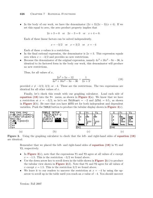
Finally, let’s check this result with our graphing calculator. Load each side of
equation (18) into the Y= menu, as shown in Figure 2(a). We know that we have
a restriction at x = −3/2, so let’s set TblStart = −2 and ∆Tbl = 0.5, as shown
in Figure 2(b). Be sure that you have AUTO set for both independent and dependent
variables. Push the TABLE button to produce the tabular display shown in Figure 2(c).
(a) (b) (c) (c)
Figure 2. Using the graphing calculator to check that the left- and right-hand sides of equation (18)
are identical.
Remember that we placed the left- and right-hand sides of equation (18) in Y1 and
Y2, respectively.
• In Figure 2(c), note that the expressions Y1 and Y2 agree at all values of x except
x = −1.5. This is the restriction −3/2 we found above.
• Use the down arrow key to scroll down in the table shown in Figure 2(c) to produce
the tabular view shown in Figure 2(d). Note that Y1 and Y2 agree for all values of
x except x = 1.5. This is the restriction 3/2 we found above.
• We leave it to our readers to uncover the restriction at x = −4 by using the uparrow
to scroll up in the table until you reach an x-value of −4. You should uncover
Version: Fall 2007