Tanga Fisheries Analysis - IUCN

IUCN Eastern Africa Regional Programme 

Analysis of reef fisheries 

under co-management in Tanga 

Jim Anderson 

December 2004 

Tanga Coastal Zone Conservation and Development Programme

Analysis of reef fisheries 

under co-management in Tanga 

Jim Anderson 

December 2004 

Tanga Coastal Zone Conservation and Development Programme 

i

The designation of geographical entities in this book, and the presentation of the material, do not 

imply the expression of any opinion whatsoever on the part of IUCN, Government of Tanzania or 

Development Cooperation Ireland (DCI) concerning the legal status of any country, territory, or area, 

or of its authorities, or concerning the delimitation of its frontiers or boundaries. 

The views expressed in this publication do not necessarily reflect those of IUCN, Government of 

Tanzania or Development Cooperation Ireland (DCI). 

This publication has been made possible in part by funding from Development Cooperation Ireland 

(DCI). 

Published by: 

Reproduction of this publication for educational or other non-commercial 

purposes is authorized without prior written permission from the copyright holder 

provided the source is fully acknowledged. 

Reproduction of this publication for resale or other commercial purposes is 

prohibited without prior written permission of the copyright holder. 

Citation: 

Anderson, J. (2004): Analysis of reef fisheries under co-management in 

Tanga, x + 51pp. 

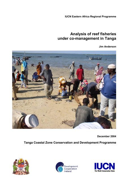
Cover photo: 

Deep-Sea Landing Site, Tanga. Jim Anderson 

Available from: 

IUCN EARO Publications Service Unit 

P. O. Box 68200 - 00200, Nairobi, Kenya 

Tel: + 254 20 890605 – 12 

Fax: +254 20 890615 

E-mail: mail@iucn.org 

ii

Table of Contents 

Acknowledgements ..................................................................................................................... vi 

Executive Summary.................................................................................................................... vii 

1. Background ............................................................................................................................. 1 

2. A Brief History of TCZCDP Collaborative Management Areas............................................. 1 

3. A summary of all available Frame Survey data for Tanga Region....................................... 3 

4. Summary Description of Previous and Current Fisheries 

Sampling Protocols in TCZCDP ............................................................................................. 4 

4.1. First TCZCDP Fisheries Sampling Protocol (1995-2001) ................................................... 5 

4.1.1. Description of the Sampling Method .............................................................................. 5 

4.1.2. Observations on the 1 st TCZCDP Sampling Protocol ..................................................... 6 

4.2. Second TCZCDP Fisheries Sampling Protocol (2001-2003) .............................................. 7 

4.2.1. Description of the Sampling Method .............................................................................. 7 

4.2.2. Observations on the 2 nd TCZCDP Sampling Protocol .................................................... 8 

4.3. Third TCZCDP Fisheries Sampling Protocol (2003-present) ............................................ 10 

4.3.1. Description of the Sampling Method ............................................................................ 10 

4.3.2. Observations on the 3 rd TCZCDP Sampling Protocol................................................... 11 

4.4. Summary Comparison of the Three TCZCDP Sampling Protocols................................... 13 

5. Previous data analysis activities and their major findings ................................................ 13 

5.1. Sampling Effort 1995-2000............................................................................................... 13 

5.2. Analysis of Catch per Unit Effort (Catch-Rate) ................................................................. 14 

6. Description of Methods for the analysis of fisheries data.................................................. 15 

6.1. Estimates of Total Catch/Value ........................................................................................ 15 

6.2. Total Catch Estimate Equation Components.................................................................... 15 

6.3. Standardising CPUE data for between-year comparisons................................................ 15 

6.4. Statistical Tests................................................................................................................ 17 

7. Results from analysis of the fisheries data......................................................................... 18 

7.1. Total Catch and Value for the Region, by District and by CMA......................................... 18 

7.2. The Spatial and Temporal profile of Fishing Effort and Catch-rate ................................... 20 

7.2.1. Annual Variations in CPUE for Ngalawa using Mishipi................................................. 20 

7.2.2. Seasonal Variations in CPUE for Ngalawas using Mishipi ........................................... 21 

7.2.3. Annual Variations in CPUE for Ngalawa using Madema .............................................. 25 

7.2.4. Seasonal Variations in CPUE for Ngalawas using Madema ........................................ 25 

7.2.5. Annual Variations in CPUE for Ngalawa using Jarife ................................................... 27 

7.2.6. Seasonal Variations in CPUE for Ngalawas using Jarife.............................................. 27 

7.3. Catch Composition........................................................................................................... 30 

7.4. Variations in Price of Fish by Species/Species Group ...................................................... 34 

7.5. The Use of Different CMAs by Local Fishers.................................................................... 40 

8. Discussion and Recommendations..................................................................................... 43 

8.1. Reduced Destructive Fishing ........................................................................................... 45 

8.2. Reduced User Conflicts/Access Issues ............................................................................ 45 

8.3. Increased Fish Stocks...................................................................................................... 45 

8.3.1. Supervision of Data Collectors..................................................................................... 47 

8.3.2. Data Management ....................................................................................................... 47 

8.3.3. Fishing Gear Definitions .............................................................................................. 48 

8.3.4. Species Identification................................................................................................... 48 

8.3.5. Harmonising Data Collection with District Fisheries Office Activities ............................ 48 

iii

9. References and further reading ........................................................................................... 49 

Appendix 1 - Vessel and Fishing Gear Descriptions................................................................ 50 

Appendix 2 - Description of Pair-wise Comparisons................................................................ 51 

List of Tables 

Table 1 - History of Management Areas/CMAs Established under TCZCDP................................... 2 

Table 2 - Profile of Reef Closures by CMA...................................................................................... 2 

Table 3 - Summary of Frame Survey Landing Site, Fisher Numbers and 

Vessel Data for Tanga Region.......................................................................................... 3 

Table 4 - Summary of Frame Survey Fishing Gear Data for Tanga Region..................................... 3 

Table 5 - Landing Sites Sampled by Fisheries Division (Tanga Region) ......................................... 4 

Table 6 - Profile of Fisheries Data collected by Fisheries Division................................................... 4 

Table 7 - TCZCDP first Fisheries Data Profile (1995-2001)............................................................. 5 

Table 8 - Landing Sites Sampled for Fisheries Data under the 2nd TCZCDP Protocol ................... 8 

Table 9 - Comparison of CPUE data from TCZCDP and Fisheries Division, 

Muheza District, 2002..................................................................................................... 10 

Table 10 - Summary Comparison of TCZCDP Sampling Protocols............................................... 13 

Table 11 - Summary Profile of possible analyses under each TCZCDP Protocol.......................... 13 

Table 12 - Annual Estimates of Catch/Value for Tanga Region, 2002-2004. * Tsh1090:1USD ..... 18 

Table 13 - Annual Estimates of Catch/Value by District, 2002-2004. * Tsh1090:1USD ................. 19 

Table 14 - Annual Estimates of Catch/Value by CMA, 2002-2004 Tsh1090:1USD........................ 19 

Table 15 - Major Species groups in Ngalawa/Mishipi Data (1st Protocol) N ~ 85 .......................... 30 

Table 16 - Major Species groups in Ngalawa/Jarife Data (1st Protocol) N ~ 70............................. 30 

Table 17 - Major Species groups in Ngalawa/Madema Data (1st Protocol) N ~ 40 ....................... 30 

Table 18 - Location of Fishing Grounds in relation to Home CMA ................................................. 41 

Table 19 - Objectives/Result Areas for Tanga CMAs .................................................................... 44 

Table 20 - Summary Table of Results from Inter-Annual CPUE Comparisons .............................. 46 

Table 21 - Vessel Codes............................................................................................................... 50 

Table 22 - Fishing Gear Codes ..................................................................................................... 50 

List of Figures 

Figure 1 - Fisheries Data Collection Form for TCZCDP (1995 TO 2001)......................................... 5 

Figure 2 - Percentage of fishing trips with zero catch by fishing gear .............................................. 6 

Figure 3 - Fisheries Data Collection Form for TCZCDP (2001 to 2003)........................................... 9 

Figure 4 - Fisheries Data Collection Form for TCZCDP (March 2003 to present).......................... 12 

Figure 5 - Mean No. of Trips Recorded Daily from Kigombe Village 1995-2000. 1995 

9 = September, 1995; 1995 11 = November 1995 etc ................................................. 14 

Figure 6 - Total Catch Estimate Equation (Anon, 2002) ................................................................ 15 

Figure 7 - Mean Trip Length (Hrs) for Ngalawa/Mishipi ................................................................. 16 

Figure 8 - Mean Trip Length (Hrs) for Mtumbwi/Madema .............................................................. 17 

Figure 9 - Mean CPUE (Kg/Gr/Trip, with 90% CI) by Year/Month for 

Kigombe (Ngalawa/Mishipi), 1995-2004 ...................................................................... 17 

Figure 10 - Mean Annual CPUE (kg/gr/trip) for Ngalawa/Mishipi 1996-2004 from Kigombe village. 

Error bars represent 90% Confidence Intervals. .......................................................... 20 

Figure 11 - Mean Annual CPUE (kg/gr/trip) for Changu Ngalawa/Mishipi 1996-2004 

(with 90% Confidence Intervals) .................................................................................. 21 

Figure 12 - Mean CPUE (Kg/Gr/Trip, with 90% CI) by Year/Month for Kigombe 

(Ngalawa/Mishipi), 1995-2004 ..................................................................................... 23 

Figure 13 - Mean CPUE (Kg/Gr/Hr, with 90% CI) by Year/Month for Kigombe 

(Ngalawa/Mishipi), 2001-2004 ..................................................................................... 24 

Figure 14 - Mean Annual CPUE (kg/gr/trip) Ngalawa/Madema (with 90% Confidence Interval) .... 25 

iv


(Ngalawa/Madema), 1995-2004 .................................................................................. 26 

Figure 16 - Mean Annual CPUE (kg/gr/trip) Ngalawa/Jarife (with 90% Confidence Interval) ......... 27 


(Ngalawa/Jarife), 1995-2004........................................................................................ 28 

Figure 18 - Mean CPUE (Kg/Gr/Hr, with 90% CI) by Year/Month for Kigombe 

(Ngalawa/Jarife), 2001-2004........................................................................................ 29 

Figure 19 - Proportion of Monthly Catch of Siganidae (Ngalawa/Mishipi) ...................................... 32 

Figure 20 - Proportion of Monthly Catch of Siganidae (Ngalawa/Madema) ................................... 32 

Figure 21 - Proportion of Monthly Catch of Lethrinidae (Ngalawa/Mishipi) .................................... 33 

Figure 22 - Proportion of Monthly Catch of Lethrinidae (Ngalawa/Madema).................................. 33 

Figure 23 - Mean Price per Kilo for Chafi 1995-2001 Kigombe (with 90% Confidence Interval)..... 34 

Figure 24 - Mean Price per Kilo for Changu 1995-2001 Kigombe (with 90% Confidence Interval) 35 

Figure 25 - Mean Price per Kilo for Taa 1995-2001 Kigombe (with 90% Confidence Interval)....... 35 

Figure 26 - Mean Catch per Trip and Price Data for Kigombe....................................................... 37 

Figure 27 - Mean Price against Mean Catch (2003/04) for each CMA........................................... 38 

Figure 28 - Sampled Fishing Activity at Upangu Reef, Mtang'ata CMA ......................................... 42 

Figure 29 - Apparent Illegal Fishing Activity at Kipwani Reef, Mwarongo-Sahare CMA................. 42 

List of Equations 

Equation 1: Standard Error (Kramer, 1956; Tukey, 1953) ............................................................. 51 

Equation 2: Calculation of Tukey's 'q' value .................................................................................. 51 

v

Acknowledgements 

I would like to thank the staff of Tanga Coastal Zone Conservation and Development Programme, 

especially Mr Solomon Makoloweka, Mr Hassan Kalombo and Dr Eric Verheij, for all their 

assistance in the preparation of this report. Many thanks also to Dr Melita Samoilys, the IUCN 

Regional Coordinator - Marine and Coastal Ecosystems, for providing useful advice and guidance 

and for help in editing this document. Mr Simon Nicholson provided guidance on statistical 

analyses. 

vi

Executive Summary 

The Tanga Coastal Zone Conservation and Development Programme (TCZCDP) started in 1994 

with the aim of enhancing the well-being of the coastal communities in the Tanga Region by 

improving the health of the coastal/marine environment that they depend on. 

The Programme is implemented by the three coastal districts of Tanga Region (Muheza and 

Pangani Districts and Tanga Municipality) in collaboration with the Regional Administrative 

Secretariat, The Ministry of Natural Resources and Tourism, and the Vice-Presidents Office 

(Environment). The Eastern African Regional Office of IUCN - The World Conservation Union, 

based in Nairobi, provided technical and managerial advice on behalf of the donor agency, 

Development Cooperation Ireland. The Programme has been implemented in four phases, Phase 1 

(1994-1997), Phase 2 (1997-2000), Phase 3 (2001-2003), and Phase 4 (2004-2006). 

One of the major activities of the Programme has been to implement Collaborative Management 

Areas (CMAs) through which community-led conservation plans are implemented and by 2001, six 

CMAs had been established covering the entire length of the Tanga Region coastline. An essential 

element in the development and monitoring of resource management plans is the information 

provided by fisheries data collected across the three districts. Fisheries monitoring has sought to 

provide data suitable to assess whether the key objective, improved fishery yields and hence 

increased income to CMA residents, has been achieved. This overall objective was to result from 

an increase in resource abundance due to Programme activities including reduced destructive 

fishing, the creation of closed areas and reduced numbers of ‘visiting’ fishers. 

Data have been collected, using three different protocols, on fish-catch, species composition, price, 

and the use of marine space by fishers. The 1 st data collection protocol was established in 1995 

and continued through to 2000 and mainly collected data from Kigombe Village located in what is 

now Mtang’ata CMA. Additional monitoring was conducted at Ushongo and Kipumbwi Villages but 

data collection at these two sites was relatively short-lived. The 1 st Protocol adopted by TCZCDP, 

using a modified version of the nationwide Fisheries Division protocol, collected data on fish catch 

(using the local Ki-Swahili taxonomy), fishing effort in terms of vessel and gear-type (although not 

including hours spent at sea), the location of fishing (using local names for fishing grounds) and 

price data. The 2 nd protocol was introduced in 2000, and after a trial period was extended to 13 

villages/landing sites across all six CMAs in existence. This protocol collected similar data but effort 

(in hours) was added to the data profile. The new protocol introduced a pre-defined species list and 

those species not on the list were recorded under a single category of ‘others’. A third protocol was 

introduced in 2003 that sought to improve the statistical validity of the fisheries data by introducing 

proper stratification to the sampling regime. Data have been managed in an Access database 

developed by TCZCDP. In addition to the fisheries-dependent monitoring, a separate (fisheryindependent) 

reef-health monitoring protocol was also established by TCZCDP. 

The key fisheries indicator chosen by TCZCDP was catch per unit effort (CPUE) or catch rate. 

CPUE is taken as an index of resource abundance: as resources increase so the catch rate would 

be expected to increase. The analyses presented in this report are based on a set of data covering 

the longest possible time-series, where sample size was sufficient, and comprised data from three 

vessel/gear combinations: ngalawa/mishipi (handline); ngalawa/madema (traps); and 

ngalawa/jarife (sharknet) from Kigombe Village. Multiple comparisons between mean annual CPUE 

for these data were undertaken using the Tukey Test (with the Kramer Modification for unequal 

sample sizes). Overall there was no clear increase year-on-year for any of the three datasets 

analysed although the datasets did show different apparent patterns in CPUE. CPUE for 

ngawala/mishipi has remained fairly constant since the start of monitoring with a significant 

increase in 2003/04 data. It remains to be seen whether this is an outlier or whether subsequent 

years will continue to show an increase in CPUE, suggesting an increase in the resources targeted 

by this vessel/gear combination. Data for ngalawa/madema showed a decline in CPUE of 

vii

approximately 30% between 1996 and 2000 but by 2003/04 CPUE had recovered to be statistically 

similar to the 1996 results. For ngalawa/jarife CPUE increased by some 70% to a peak in 2000/01, 

only to fall again to be at a statistically similar level in 2003/04 compared with data from 1996/97. 

To determine whether fishery-related incomes had increased over the course of the Programme 

data on mean price per kilogramme, and mean revenues (obviously linked directly to CPUE) were 

analysed. Since the inception of TCZCDP the value of the Tanzanian Shilling has declined against 

the US Dollar, and mean price data was therefore indexed against the exchange-rate in 1996. The 

analysis for Kigombe village only indicated a decline in mean price per kilogramme of fish landed 

particularly from 1995 to 1998. The pattern observed suggests price may be partly determined by 

supply, with the decline in price in early years occurring when catch rates increased. It was not 

possible to determine any further fisheries-related income benefits to residents of the CMA. 

To monitor the use of marine space by fishers (both residents and visiting fishers), and to inform 

stakeholders on potential approaches to resolve spatial-conflicts between users of different gears, 

the location of fishing was recorded for all sampled fishing trips. Analyses were restricted because 

the majority of the data available reported on fishers from Kigombe Village only, and therefore 

could not more fully describe fishing patterns in all six CMAs. However, analysis of data, covering 

all CMAs, did indicate that there was some level of (un-restricted) migration of fishers between 

CMAs and that some important fishing grounds were probably trans-boundary and thus shared by 

fishers from different CMAs. This has implications for estimating yields and revenues from 

individual CMAs and for potentially restrictive management activities on any of these shared 

grounds. More detailed analyses will require the Programme’s vessel registration system to be 

finalised. 

A number of recommendations were offered to the Programme as the responsibility for 

management is transferred from the IUCN-supported phases to a District-managed future. 

Objective/Management 

Issue 

Monitoring Fisher 

Migrations 

Monitoring Resource 

Abundance 

Data Collection 

Mainstreaming with 

Government Protocols 

Fishery-Related Recommendation 

Complete the mapping of the fishing grounds with local 

fishers and enter into the GIS system available at 

TCZCDP HQ. 

Develop a registration system for fishing vessels and 

modify data collection form/database to allow recording 

of the registration number and therefore the home 

CMA/District of each vessel. 

Investigate alternative means of objectively verifying 

increases in fish abundance. 

A programme of field supervision, regular training 

updates for field staff and unannounced site visits 

should be established. 

There is an urgent need for a sampling and information 

management post to be created within the TCZCDP 

administration. 

Review fishing gear definitions 

Initiate discussions with District Government/Fisheries 

Division on harmonising data collection activities within 

the Tanga Region 

viii

1. Background 

The Tanga Coastal Zone Conservation and Development Programme started in 1994 and aims to 

enhance the well-being of the coastal communities in the Tanga Region by improving the health of 

the coastal/marine environment that they depend on, and by diversifying the options for the use of 

the coastal/marine resources. The Programme is working with the coastal fishing villages to 

improve management of the coral reefs and mangroves, and the coastal resources that the 

villagers depend upon for their livelihoods. Districts and village level institutions are being 

strengthened so that they can undertake integrated management in a sustainable way. 

The Programme is implemented by the three coastal districts of Tanga Region (Muheza and 

Pangani Districts and Tanga Municipality) in collaboration with the Regional Administrative 

Secretariat, The Ministry of Natural Resources and Tourism, and the Vice-Presidents Office 

(Environment). The Eastern African Regional Office of IUCN – The World Conservation Union, 

based in Nairobi, provides technical advice and manages the Programme on behalf of the donor 

agency, DCI. The Programme has been implemented in four phases, Phase 1 (1994-1997), Phase 

2 (1997-2000), Phase 3 (2001-2003), and Phase 4 (2004-2006). 

The overall Goal of Phase 4 of the Programme is: “Integrity of the Tanga coastal zone ecosystem 

improved, and its resources supporting sustainable development”. The Purpose is: “Improved 

coastal zone resources management by District Administration, resource users, and other 

stakeholders”. 

Three results were identified by which the Goal and Purpose would be achieved: 

• Strengthening institutional support for long-term implementation of collaborative 

management area plans. 

• Strengthening of knowledge base and supporting decision-making and adaptive 

management. 

• Programme effectively managed, monitored, and evaluated. 

An essential element in the development, and monitoring, of resource management plans is the 

information provided by fisheries data collected across the three districts. The data collection 

protocol has been adapted since the Programme’s inception in 1994 and the most significant 

modification took place in January 2002. 

A more detailed analysis of the fisheries data was required in order to better determine the effect of 

the management plans and their associated activities. This consultancy therefore undertook a 

thorough review of all historical protocols, an analysis of the available fisheries data, and provides 

some recommendations on future monitoring protocols. The Terms of Reference are presented in 

Appendix 3. 

2. A Brief History of TCZCDP Collaborative Management Areas 

The collaborative management areas of TCZCDP have undergone some modification in their 

boundaries, and been re-named since the inception of the Programme. The original profile of what 

were known as village management plans (Horril et al., 2001) and the current profile of what 

became known as Collaborative Management Areas (CMA) (TCZCDP, pers. comm.) are presented 

in Table 1. Note in Table 1 that there is usually a gap between the time the management 

areas/plans are developed and the time they are approved. In fact the area management plans 

have to be approved at three of the levels of governance under which TCZCDP operates following 

adoption by the respective village councils. These three authorities are: 

1

• The local Central Coordinating Committee (CCC); 

• The District Council(s) in which the management area in located; and, 

• The Fisheries Division in Dar es Salaam. 

There have also been three reviews of each management area plan (which have taken place at 

different times for each CMA), and again the three levels of approval are required (TCZCDP, pers. 

comm.). 

Table 1 - History of Management Areas/CMAs Established under TCZCDP 

Name of Villagebased 

Management 

Plan 

Kigombe-Tongoni 

Boza-Sange 

Ushongo-Sange 

Date of 

Development 

(Approval) 

July 1996 

(1997) 

September 1996 

(1997) 

July 1998 

(1999) 

Developed or 

Incorporated 

into 

Name of 

Collaborative 

Management Area 

(CMA) 

Date of 

Development 

(Approval) 

→ Mtang’ata* 1999 

→ 

Boza-Sange 

Mwarongo-Sahare 

Mkwaja-Sange 

Deep Sea-Boma 

Boma-Mahandakini 

1999 

(2000) 

July 1999 

(2000) 


(2001) 


(2001) 

2000 

(2001) 

* Mtang’ata is the only CMA that straddles two districts (Muheza and Tanga Municipality). 

Under these various plans there have been a number of specific fisheries-related management 

activities principle amongst which is the reduction or elimination of the use of dynamite (which is in 

any case illegal in Tanzania), and the establishment, with full stakeholder participation, of closed 

areas. Table 2 presents a summary of the reefs that have been closed and identifies those that 

have subsequently re-opened to fishing. 

Table 2 - Profile of Reef Closures by CMA 

CMA 

Reef Name 

Date of 

Closure 

Current 

Status 

Date of Opening 

Boma-Mahandakini Bunju 2001 Closed 

Deep Sea-Boma Chundo/Kiroba 2000 Closed 

Mwarongo-Sahare Kipwani 2000 Closed 

Kitanga 1996 Open 1999 

Mtang’ata 

Makome 2001 Closed 

Shenguwe 2001 Closed 

Upangu 1996 Open 1999 

Boza-Sange 

Mkwaja-Sange 

Dambwe 1998 Closed 

Maziwe 1975 Closed 

No Closures 

2

3. A summary of all available Frame Survey data for Tanga Region 

A frame survey is defined as ‘a complete description of the structure of any system to be sampled for collection of 

statistics. In fisheries, it may include the inventory of posts, landing places, number and type of fishing units (boats 

and gears), and a description of fishing and landing activity patterns, fish distribution routes, processing and marketing 

patterns, supply centres for goods and services, etc.’ (Modified from Anon, 2002). 

The data on the number and type of fishing units generated by a frame survey is used in 

conjunction with sample fisheries data (catch/effort/value etc collected at landing sites/markets etc) 

to estimate the total catch/effort/value of that particular system. The sample data (average catch 

per gear-hour, for example) is raised by multiplying it by the frame survey data to give the total 

catch for that fleet/gear type. For example, in basic terms, if the average catch of a ring-net is 50kg 

per gear-hour (from sample data), the average trip length is 5 hours (from sample data), all the 

ring-nets in the fleet are used every day of the month (from sample data) and there are 100 ringnets 

of this type in the fleet (from the frame survey data), then the total catch per month for that 

fleet will be estimated as 50kg*5hrs*30days*100nets = 750,000kg. A similar exercise could be 

undertaken for beach-seine nets, or fish traps, using sample data and frame survey data specific 

for those types of gears. 

Marine frame surveys were undertaken by the Fisheries Division in 1995, 1998 and most recently 

in 2001 and the data from these are presented in Table 3 and Table 4. 

Table 3 - Summary of Frame Survey Landing Site, Fisher Numbers and Vessel Data for Tanga Region 

Year 

No. of 

Landing 

Sites 

Number of 

Fishers* 

Number of 

Engines** 

Vessel Categories 

IB OB Ngalawa Mashua Mtumbwi Dau Boti 

1995 48 4,202 2 96 394 150 261 50 41 

1998 46 4,380 2 95 452 84 262 137 34 

2001 52 4,361*** 5 91 502 100 237 84 21 

Source: Fisheries Division 

* Includes those recorded as ‘owners’. 

** IB = Inboard Engine; OB = Outboard Engine 

*** Numbers of fishers were adjusted to account for apparent anomalies in some landing site datasets between 1998 and 

2001. 

Table 4 - Summary of Frame Survey Fishing Gear Data for Tanga Region 

Year 

Gill-net 

Shark 

Net 

Handline 

Longline 

Beach 

Seine 

Fish 

Traps 

Ring 

Nets 

Scoop 

Nets 

1995 1,182 814 2,898 38 57 1,294 79 66 

1998 631 608 2,654 34 84 1,258 128 255 

2001 953 404 1,883 56 a - b 2,161 102 106 


a 

The frame survey reports 788 longlines for 2001 but this is an error – data recording mixed number of hooks per line 

with number of lines (H. Kalombo pers. comm.). When recalculated from the raw data the actual figure is around 56 (33 

in Muheza, 23 in Pangani and 0 in Tanga) 

b Beach seines were banned in 2001. 

3

4. Summary Description of Previous and Current Fisheries Sampling Protocols in 

TCZCDP 

Why Sample? Sometimes, the entire population will be sufficiently small, and the researcher can include the entire 

population in the study. This type of research is called a census study because data is gathered on every member of 

the population. Usually, the population is too large for the researcher to attempt to survey all of its members. A small, 

but carefully chosen sample can be used to represent the population. The sample reflects the characteristics of the 

population from which it is drawn. (Source: Statpac Survey Software, Sampling Methods) 

In order to know whether management activities are having the desired affect in terms of improving 

incomes of small-scale fishers or increasing the abundance of particular species (etc.), managers 

need to have information from the fishery itself. But obtaining information on every catch landed or 

price obtained etc from fishers is usually impractical because it is expensive and time-consuming, 

especially in small-scale fisheries where there are many small, isolated landing sites often with 

poor access. So sampling protocols are usually developed, which give a statistically accurate 

picture of the fishery but only require a certain number of fishing trips to be recorded. These 

sample data are then used in conjunction with the frame survey data (as described in Section 3) to 

estimate total catch/revenue. 

There have been three distinct sampling protocols employed under the TCZCDP. At the time of 

inception of TCZCDP the Fisheries Division operated a sampling regime at six landing sites in 

Tanga Region (see Table 5). 

Table 5 - Landing Sites Sampled by Fisheries Division (Tanga Region) 

Landing Site 

Moa 

Kwale 

Kigombe 

Tongoni 

Deep Sea 

Kipumbwi 


District 

Muheza 

Muheza 

Muheza 

Tanga 

Tanga 

Pangani 

A range of data were (and continue) to be collected and these are presented in Table 6. The 

sampling methodology was based on 16-days sampling per month at the six sites with an expected 

100% coverage of the fishing activities on those days, i.e. all boats that land a catch on a given 

sampling day should be interviewed and the catch/effort recorded. Note that data were not 

collected according to scientific nomenclature but using local taxonomy, which tends to group a 

number of species and genera (and in some cases families) together under species groupings. 

Table 6 - Profile of Fisheries Data collected by Fisheries Division 

Effort Data 

Date 

Vessel Registration Number 

Vessel Type 

Gear Type, Number and size 

Number of Crew 

Arrival Time 

Time Spent Fishing 

Catch Data 

Weight by species (groupings) 

Number by species (groupings) 

Economic Data 

Value of catch (beach price) by species (groupings) 


4

Although this profile is a useful one for fisheries data, there was typically a limited level of 

supervision of monitors, and, equally crucial, the data management was poor to the extent that 

these raw data, apart from summary profiles in Annual Reports, are no longer available to 

researchers. Although an ACCESS database had been developed in 2002 under the RFIS Project 

(SADC/DFID) to facilitate the entry, production analysis and reporting of data, the up-take of this 

system and hence the opportunities for improved data management were limited. 

4.1. First TCZCDP Fisheries Sampling Protocol (1995-2001) 

With the inception of the TCZCDP there was an attempt to improve on the Fisheries Division data 

collection system and to take some control over the data that was collected. 

4.1.1. Description of the Sampling Method 

The first protocol modified the Fisheries Division data collection form, and TCZCDP-seconded staff 

collected the data. These were collected at the market place rather than at the actual landing-site. 

A similar sampling protocol to that used by the Fisheries Division was employed (16-days per 

month, 100% coverage of fishing trips on those days) but the data profile was adjusted and effort 

was no longer recorded. The data profile is shown in Table 7. 

Table 7 - TCZCDP first Fisheries Data Profile (1995-2001) 

Effort Data 

Date 

Name of Fisher 

Vessel Type 

Gear Type and Number 

Place of Fishing 

Catch Data 

Weight by species (species groupings) 

Number by species (species groupings) 

Economic Data 

Value of catch (beach price) by species (groupings) 

Source: TCZCDP 

The first village management plan was established under TCZCDP in Kigombe-Tongoni, off 

Muheza District (see Table 1) and the 1 st sampling protocol was implemented at the Kigombe 

landing site on the 30 th September, 1995. Further data collection activities were established at 

Kipumbwi village, for the adjacent Ushongo-Sange village management plan from August 1996 to 

September 1999 and at Ushongo village (Boza-Ushongo village management plan), from May to 

September 1999. Figure 1 presents a short-version of the data collection form used under the 1 st 

Protocol. 

Figure 1 - Fisheries Data Collection Form for TCZCDP (1995 TO 2001) 

Date 

Name of 

Fisher 

Type of 

Boat 

Gear (No.) 

Name of 

Fishing 

Ground 

Type of 

Fish 

Number of 

Fish Weight Value 


The database holding the 1995-2001 data has an additional category of fisheries-related data to 

those collected on the form shown in Figure 1, namely size category and number of fish within 

each category. There are three categories, A, B, and C (originally a fourth category was also used) 

which relate respectively to the length of a hand, the length from fingertip to mid-forearm and the 

length from fingertip to shoulder. 

5

Mishipi Madema Nyavu RingNet Jarife Kaputi 

4.1.2. Observations on the 1 st TCZCDP Sampling Protocol 

There are many types of data that can be taken during sample surveys (mean catch, trip length, 

revenue per trip, the species composition, the fishing ground used, the weather, the time of fishing 

etc). These data can be used for a range of purposes. One of the most common uses of the catch 

and effort data is to calculate the catch per unit effort. 

Catch-Per-Unit-Effort (CPUE) - also called catch rate - is frequently the single most useful index for long-term 

monitoring of a fishery. Declines in CPUE may mean that the fish population cannot support the level of harvesting. 

Increases in CPUE may mean that a fish stock is recovering and more fishing effort can be applied. 

CPUE can therefore be used as an index of stock abundance, where some relationship is assumed between that 

index and the stock size. Catch rates by boat and gear categories, often combined with data on fish size at capture, 

permit a large number of analyses relating to gear selectivity, indices of exploitation and monitoring of economic 

efficiency. (Source: Anon, 2002). 

There are three issues on the use of CPUE related to the 1 st Sampling Protocol: 

• No fishing effort, except ‘fishing trip’, was recorded: Managers/researchers would be 

looking to observe what happens to the CPUE over time, that might reflect an increasing, 

stable or decreasing abundance of fish. However, without details on the actual fishing effort 

(ideally numbers of hours) other than numbers of trips it is possible that a change in CPUE 

(catch per trip) will not accurately reflect the abundance of fish because trip length may 

have changed and so fishers may be spending more (or less) time at sea to catch a given 

amount of fish. 

• Data were collected at the market place rather than at the landing site beaches: Recording 

catch data at the market place means that no zero-catches would be recorded (because 

fishers would not have anything to sell) and this would give a false-impression of the CPUE 

information. The impact of this omission depends somewhat on the gear one is talking 

about and a graphical display of the variation between gears is presented in Figure 2. 

Figure 2 - Percentage of fishing trips with zero catch by fishing gear 

Percentage of fishing trips where a zero catch was 

recorded 

100 

90 

80 

Percentage of Trips 

70 

60 

50 

40 

30 

20 

10 

0 

Fishing Gear 

Zero Catch Recorded 

Catch > 0kg Recorded 

Data source: TCZCDP 

6

• An issue related to the market-based sampling is that smaller catches, both in size of fish 

and weight, would not tend to be auctioned at market (where a levy is charged) but would 

have been sold on the landing beach. If small catch/zero-catches are not recorded this will 

give a misleading figure for the CPUE: it will have the effect of increasing the mean CPUE 

because only larger (auctioned at market) catches will be recorded. The amount and 

quality of data collected in market-based sampling may be reduced because of the speed 

at which catches are sold-off, and the fact that potential buyers, or the vendors themselves, 

do not usually want researchers handling their catch. This creates a challenge for data 

collectors, who generally rely on the good-will of fishers/vendors, to satisfactorily complete 

their work. This is by no means a simple problem to solve and beach sampling also faces 

similar challenges because fishers are usually keen to get their catch processed and sold 

quickly with minimal interference from data collectors or other researchers. 

A further important feature of this 1 st 

designed into the sampling. 

Protocol was that there appeared to be no stratification 

Stratified sampling is commonly used probability method that is superior to random sampling because it reduces 

sampling error. A stratum is a subset of the population that share at least one common characteristic. Examples of 

stratums might be dhows and ngalawas, or mishipi and nyavu. The researcher first identifies the relevant stratums and 

their actual representation in the population. Random sampling is then used to select a sufficient number of subjects 

from each stratum. "Sufficient" refers to a sample size large enough for us to be reasonably confident that the stratum 

represents the population. Stratified sampling is often used when one or more of the stratums in the population have a 

low incidence relative to the other stratums. (Modified from Statpac Survey Software, Sampling Methods) 

A somewhat unusual feature of the data generated under this first protocol, given that small-scale 

reef fisheries tend to be multi-species in profile, is that relatively few trips appear to have caught 

more than one species (or group). In fact only 9% of all the fishing trips recorded having more than 

one species/species group, compared to 24% in the more recent data collected by TCZCDP. The 

reason for this is not specifically understood but it may originate in the design of the data collection 

form itself. 

Ideally a data form should represent the relational nature of the information required from a fishing 

trip; that is to say that one fishing trip (the effort, including date, time, area fished, type of boat etc) 

will relate to more than one record of catch (i.e. there are usually more than one species caught in 

a single trip). But the original design nominally allows for only one row of information per trip. If 

more than one species is actually recorded then more than one row will have to be entered, 

although this can result in duplicate date, time, and area fished etc being entered, or just empty 

cells. This can lead data collectors to just write a single record for each trip, rather than fill in the 

entire catch. Neither does such a form design facilitate the data entry process (because of the 

empty cells or duplicate data). 

4.2. Second TCZCDP Fisheries Sampling Protocol (2001-2003) 

The second data collection protocol employed by TCZCDP was initiated by the newly appointed 

Technical Advisor (TA) in June 2000. In addition to issues related to statistical design, the TCZCDP 

had also moved from what was a village-based pilot programme to an area-based management 

approach. This change in design necessitated a larger-scale monitoring programme to be 

developed (Hassan Kalombo, TCZCDP, pers. comm.). 


This protocol was first piloted in August 2001. The villages that were sampled are presented in 

Table 8. The design was based on sampling in three-four villages per district, with each village 

sampled once every three-months. The protocol attempted to sample at least 20% of each 

category of vessel present at the landing site on any sampling day (TCZCDP, pers. comm.). 

The improved data entry form (translated into English) is presented in 

7

Figure 3. 

Table 8 - Landing Sites Sampled for Fisheries Data under the 2nd TCZCDP Protocol 

Management Area Village/Landing site (period 

sampled) 


Moa; Moa/Kijiru (2002-present) 

Kipumbwi (2002-present) 

Boza-Sange 

Pangani (2002 only) 

Stahabu (2003-present 

Ushongo (2002 only) 

Deep-sea (2002-present) 

DeepSea-Boma 

Kichalikani (2002-present) 

Mwandusi (2002 only) 

Mkwaja-Sange 

Mtang’ata 

Mkwaja (2002-present) 

Kigombe (2001-present) 

Machui (2002-present) 



Mwarongo (2002-present) 

Sahare (2002-present) 

4.2.2. Observations on the 2 nd TCZCDP Sampling Protocol 

This 2 nd Protocol included a number useful changes compared with the 1 st Protocol: 

• Sampling took place in a larger number of villages covering all the so-called Collaborative 

Management Areas (CMAs) that were then in place; 

• An attempt was made at incorporating some degree of stratification by recording 20% of 

the catches from each vessel-type although this does put an unnecessary onus on the data 

collectors to make decisions about their sampling activity; 

• Effort (in hours) was recorded; 

• Sampling was conducted on the beach (rather than in the market); 

• The data form targets pre-determined species for the detailed sampling of weight and 

numbers. The rationale for this is not clear; 

• The design of the data collection form conforms to the requirement that the relational (oneto-many) 

nature of data generated from a single fishing trip is effectively captured on the 

data collection form; 

• There was no option to record price data for individual species unlike under the 1 st 

Protocol. 

8

Figure 3 - Fisheries Data Collection Form for TCZCDP (2001 to 2003) 

Fish Catch Recording Data Sheet 

O Boza-Sange 

O DeepSea-Boma 

Village:………………… 

O Mtang’ata 

O Boma-Mahandakini 

Recorder:………………….. 

O Mwarongo-Sahare 

O Mkwaja-Sange 

Date: / / Time: ……… 

Name of Skipper/Fisher: ………………………………..Number of Fishers:…………………………… 

Type of Boat: O Ngalawa O Canoe O Dau O Mashua 

Type of Gear: ……………… …………………………Number of Gears:………………………………. 

Name of Fishing Ground:………………………… Time spent fishing:…………………..Hrs 

Total Weight of Fish: ………Kg O Estimated O Weighed 

Total Number of Fish: …… O Estimated O Counted Value (Tshs):……… 

Changu (Snappers & Emperors) Pcs Kg 

Changu Doa (L.harak) Pcs Kg 

Changu Njana (L.lentjan) Pcs Kg 

Mkundaji (Goatfish) Pcs Kg 

Mkundaji 1 (P.cinnabarinus) Pcs Kg 

Mkundaji 2 (P.indicus) Pcs Kg 

Chafi (Rabbitfish) Pcs Kg 

Chafi (S.luridus) Pcs Kg 

Chafi (S.sutor) Pcs Kg 

Kangu Pcs Kg 

Kangu 1 (S.ghobban) Pcs Kg 

Kangu 2 (H.harid) Pcs Kg 

Mlea (Sweetlips) Pcs Kg 

Mlea (P.gaterinus) Pcs Kg 

Kohe (D.pictum) Pcs Kg 

Mbono (Fusiliers) Pcs Kg 

Mbono 1 (C.xanthonotus) Pcs Kg 

Mbono 2 (C.diagramma) Pcs Kg 

Chewa (Groupers) Pcs Kg 

Chewa (E.fasciatus) Pcs Kg 

Mjombo (E.punctatus) Pcs Kg 

Taa (Rays) Pcs Kg 

Taa (D.jenkinsii) Pcs Kg 

Pungu (S.narinari) Pcs Kg 

Jodari (Tuna) Pcs Kg 

Kibua/Bangra (R.kanagurta) Pcs Kg 

Jodari (T.albacarus) Pcs Kg 

Mizia ( Barracudas) Pcs Kg 

Mizia (S.barracuda) Pcs Kg 

Msusa (P.fosteri) Pcs Kg 

Kolekole (Jacks) Pcs Kg 

Kolekole manjano (C.sem) Pcs Kg 

Kolekole ubwi (C.sexfasciatus) Pcs Kg 

Note that Changu were listed as comprising only snappers (Lutjanidae) although the species listed on the form are 

emporers (Lethrinidae). Although the TCZCDP had developed their own various data collection protocols, the Fisheries 

Division of Tanzania continued to collect their own data independently of TCZCDP. A quick comparison of data for three 

months in 2002, collected in Muheza District, against the TCZCDP data reveals the extent of the differences between 

estimates of CPUE (kg per gear-hour) derived from the two sources (seeTable 9) and see Appendix 1 for definition of 

gear types and of boat types. 

9

Table 9 - Comparison of CPUE data from TCZCDP and Fisheries Division, Muheza District, 2002 

Year 

(2002) 

Type of 

Fishing 

Gear 

TCZCDP 

Mean Catch 

(kg/gr-hr) 

Fisheries 

Division 

Mean Catch 

(kg/gr-hr) 

FD Data >10% 

Higher or Lower 

than TCZCDP? 

Type of 

Month Boat 

2 DC Mi 0.64 0.66 - 102.5% 

FD Data as % of 

TCZCDP Data 

2 DH Ny 0.20 0.12 L 62.2% 

2 DH Ja 0.92 0.58 L 62.8% 

2 DH Ma 0.79 0.20 L 25.2% 

2 NG Mi 0.38 0.40 - 106.7% 

3 NG Mi 0.27 0.35 H 129.8% 

4 DC Ny 0.32 0.07 L 21.9% 

4 DH Ny 0.22 0.07 L 32.4% 

4 DH Ja 0.62 0.28 L 45.6% 

4 NG Ny 0.32 0.07 L 21.3% 

4 NG Mi 0.30 0.18 L 59.9% 

4 NG Ja 0.81 1.04 H 127.6% 

5 DC Ny 3.22 0.08 L 2.4% 

5 DH Ny 0.54 0.08 L 14.2% 

5 DH Mi 0.53 0.36 L 67.2% 

5 DH Ja 0.59 0.52 L 88.1% 

5 NG Mi 0.50 0.29 L 58.7% 

4.3. Third TCZCDP Fisheries Sampling Protocol (2003-present) 

The third fisheries data collection protocol employed by TCZCDP was developed in collaboration 

with the SADC/RFIS Project and established in March 2003. 


This 3 rd protocol was specifically designed to report on monthly catches/revenues by district and 

vessel/gear combination, in preparation for a district-based fisheries permit system and therefore 

district and month is the major stratum, and vessel/gear combination the minor stratum against 

which the sampling was planned. The FAO publication ‘Sample-Based Fishery Surveys – A 

Technical Handbook’ (Anon, 2002) was employed to develop the survey protocol, based on the 

approach of sampling in space and in time. The sampling was marginally constrained by the fact 

that it had to take place at the same landing sites as presented in Table 8. The required sample 

size for each stratum was defined as the target for each vessel/gear combination to achieve 90% 

accuracy in the data (Anon, 2002) and therefore depended on the estimated population size 

(maximum number of trips likely per month within a district, by vessel/gear combination) but 

typically ranged between 30-32 samples per month. The selected villages were then apportioned 

sampling effort in order that the required sample sizes for each vessel/gear combination were 

achieved. Because this 3 rd Protocol was developed according to the FAO Guidelines, it is possible 

to utilize the full equation to calculate an estimate of total catch for a stratum. The modified version 

of the data collection form is presented in Figure 4. Note that a space was provided on the new 

form for the collection of length-frequency data, although at the time of writing a sampling protocol 

for length-frequency data had not yet been implemented. 

In order to obtain the necessary data for raising catch/effort samples to estimate the total catch for 

the stratum the 3 rd Protocol form design also included Boat Activity Coefficient (BAC) data. One 

can’t necessarily assume that every fisher goes fishing everyday and BAC data reports on the 

individual choices made by fishers about whether to fish or not on any particular day. They may 

have other things to do, such as farming activities. Following the FAO Guidelines the approach 

taken was of asking sampled fishers whether they had fished the three-days prior to the date of 

that particular interview. This is a cost-effective and efficient way of obtaining the necessary sample 

size (according to FAO this is three-times the sample size required for the fisheries catch/effort). A 

10

further requirement for raising catch/effort samples is a record of a fleet’s Active Days, i.e. how 

many days an entire fleet is active during the month, perhaps fishing is prevented due to a storm, 

or a religious holiday. This data is reporting an influence that tends to affect the whole fleet. This 

data can be generated through a few interviews with key informants at the end of each month of 

sampling and a separate form was provided to TCZCDP to record this data. TCZCDP were 

previously assuming, based on their own knowledge of the fisheries, that approximately 21-days 

were fished each month (TCZCDP, pers. comm.). 

4.3.2. Observations on the 3 rd TCZCDP Sampling Protocol 

• Building on the 2 nd Protocol, but with improved stratification of sampling; 

• Sampling protocols (number of samples required from each sample site by vessel-type and 

gear) were produced and issued to data collectors to rationalize sampling effort; 

• The introduction of Boat Activity Coefficient (BAC) and Vessel Activity Survey (VAS) offers 

data managers a more robust means of estimating total catch/revenues by sampling 

stratum. However, data management activities within TCZCDP should include adequate 

support to data collectors to ensure that sampling requirements are met at each site; 

• The introduction of options for collecting Length-frequency data on the same form (rather 

than having a separate form) is useful because it ensures LF samples will be attributable to 

a particular fishing trip/vessel/gear/fishing ground etc; 

• The 3 rd Protocol doesn’t allow for species/species group price data to be collected unless 

the catch is entirely single species; 

• The selection of the species list printed on the data sheet could be re-visited in light of the 

dominant species in the catch and the inclusion of species that are relatively uncommon in 

the catch. 

11

Figure 4 - Fisheries Data Collection Form for TCZCDP (March 2003 to present) 

Fish Catch Recording Data Sheet 

Village:………………… Recorder:………………….. Date: / / Time: ……… 

Name of Fisher: ……..…………………………………… Number of Crew:…………………………… 

Type of Boat: O Ngalawa O Canoe O Dau O Mashua 

Type of Gear: ……………… …………………………Number of Gears:……………………………. 

Fishing Ground:……………………………… Time Spent Fishing:…………………..Hrs 

Weight of Fish:…………………KG O Estimated O Weighed Value:……… 

Number of Fish:………………… O Estimated O Actual Value 

BAC Survey Day -3: y / n Day -2: y / n Day -1: y / n 

Type of Fish 

Length 

(cm) 

Type of Fish PCS KG 

Changu (Snappers & Emperors) 

Changu Doa (L.harak) 

Changu Njana (L.lentjan) 

Mkundaji (Goatfish) 

Mkundaji 1 (P.cinnabarinus) 

Mkundaji 2 (P.indicus) 

Chafi (Rabbitfish) 

Chafi (S.luridus) 

Chafi (S.sutor) 

Kangu 

Kangu 1 (S.ghobban) 

Kangu 2 (H.harid) 

Mlea (Sweetlips) 

Mlea (P.gaterinus) 

Kohe (D.pictum) 

Mbono (Fusiliers) 

Mbono 1 (C.xanthonotus) 

Mbono 2 (C.diagramma) 

Chewa (groupers) 

Chewa (E.fasciatus) 

Mjombo (E.punctatus) 

Taa (Rays) 

Taa (D.jenkinsii) 

Pungu (S.narinari) 

Jodari (tuna) 

Kibua/Bangra (R.kanagurta) 

Jodari (T.albacarus) 

Mizia ( Barracudas) 

Mizia (S.barracuda) 

Msusa (P.fosteri) 

Kolekole (Jacks) 

Kolekole manjano (C.sem) 

Kolekole ubwi (C.sexfasciatus) 

12

4.4. Summary Comparison of the Three TCZCDP Sampling Protocols 

Table 10 presents a summary comparison of the three TCZCDP sampling protocols according to a 

number of criteria related to statistical robustness and utility for fisheries management analysis. 

Table 10 - Summary Comparison of TCZCDP Sampling Protocols 

Sampling Protocol 

Speciesspecific 

Price 

Data? 

Compatibility 

with FAO 

Guidelines 

Stratified? 

Detailed 

Effort 

Sampled? 

Zero- 

Catches? 

Sampling 

at Beach 

Landing 

Site 

1 st (1995-2000) Y N N N N N 

2 nd (2001-2003) N N Y/N Y Y Y 

3 rd (2003-present) N Y Y Y Y Y 

Taking the observations in Table 10, it is possible to provide a summary profile of the types of 

analysis that are possible with the data generated under each data collection protocol and this is 

presented in Table 11. 

Table 11 - Summary Profile of possible analyses under each TCZCDP Protocol 

Sampling 

Protocol 

Speciesspecific 

Price 

Analysis 

Analysis of 

Catch by 

Vessel/Gear 

Analysis of 

use of 

Fishing 

Grounds 

Detailed 

CPUE 


Accurate 

estimate of 

catch/effort by 

stratum 

Length- 

Frequency 

Distribution 


1 st (1995- 

2000) 

Y Y Y N N N 

2 nd (2001- 

2003) 

N Y Y Y N N 

3 rd (2003- 

present) 

N Y Y Y 

Y 

(with improved 

data collection) 

Y 

(when a 

protocol is 

introduced) 

5. Previous data analysis activities and their major findings 

One of the principle reports of analyses of data on TCZCDP marine resources was prepared by 

Horrill et al. (2001), which covered data from 1995 to 2000. As far as it relates to fisheries there 

were a number of issues covered, including observations on controls of fishing effort at Kigombe, 

which was the main sample site during the early years of the programme. 

5.1. Sampling Effort 1995-2000 

Figure 5 presents data on the mean daily number of trips recorded from Kigombe Village, 1995- 

2000. These data indicate a decline in the coverage of the sampling and Horrill et al. (2001) 

suggested that this might be the result of reduced numbers of fishing trips by all fishers (because 

coverage was designed as 100% of fishing trips on each sampling day), reduced numbers of 

visiting fishers from outside the management area, or that it might be an attempt by fishers to avoid 

13

the fish levy at the market place. The former would suggest some considerable success in reducing 

numbers of visitors but would also have required that permission was not being granted to visiting 

fishers, while the latter has to be put into the context of the taxation system, and the question 

asked why has the change occurred from around mid-1997? Unfortunately data are unavailable to 

determine which, if in fact either of these is responsible. 

Figure 5 - Mean No. of Trips Recorded Daily from Kigombe Village 1995-2000. 1995 9 = September, 

1995; 1995 11 = November 1995 etc 

Mean Number of Trips Recorded from kigombe Landing Site 

1995-2000 

30 

25 

20 

15 

10 

5 

0 

1995 9 

1995 11 

1996 1 

1996 3 

1996 5 

1996 7 

1996 9 

1996 11 

1997 1 

1997 3 

1997 5 

1997 7 

1997 9 

1997 11 

1998 1 

1998 3 

1998 5 

1998 7 

1998 9 

1998 11 

Mean Number of Trips 

Recorded Daily 

1999 1 

1999 3 

1999 5 

1999 7 

1999 9 

1999 11 

2000 1 

2000 3 

Year/Month 

5.2. Analysis of Catch per Unit Effort (Catch-Rate) 

There are various analyses of catch rate data presented in the Horrill et al. report, including: 

• Catch per gear for pull-seine nets (before they were banned in 2000) showed ‘the greatest 

increase’ (Horrill et al., 2001, page 17); 

• Handlines showed a smaller increase in catch per gear relative to pull-seine nets (p17); 

• Entanglement nets (shark nets or jarife) showed a smaller increase in catch per gear 

relative to handlines (p17); 

• Catch per gear for gill-nets was reported as ‘stable’ (p17); 

• Catch per gear for fish-traps indicated a ‘steady decline’ (p17). 

However, these interpretations are complicated by a number of issues. No statistical analyses are 

given that might determine whether the increases in catch per gear was in fact significantly 

different. Without detail on the time spent fishing it is impossible to say whether there is an increase 

in catch per gear (i.e. an increase in abundance of fish) or whether the fishers are just spending 

more time fishing (with or without the same number of gears). Details on effort allow for identifying 

more subtle changes in fishing practice. For example, it is possible that in 1995 a fisher deployed 

his/her two entanglement nets for one-hour (i.e. two gear-hours) to generate a total catch of 5 kg at 

a rate of 2.5kg per gear-hour, and 2.5kg per gear per trip; while in 2000 the fisher deployed the 

same two nets for two-hours (i.e. four gear-hours), and caught 10kg, still therefore only at a rate of 

2.5kg per gear-hour (i.e. indicating the same abundance of fish), but at a rate of 5kg per gear per 

trip. This is misleading because it suggests an increase in catch-rate (i.e. fish abundance) but in 

fact it required the fisher deploy the gear in 2000 for twice as long as in 1995, that is to say there 

has been no net increase in kg/gr/hr, a more accurate unit for CPUE, than kg/gr/trip. 

14

6. Description of Methods for the analysis of fisheries data 

6.1. Estimates of Total Catch/Value 

In order to estimate total catch/total value for districts/CMAs a simple equation was utilized (Figure 

6). Estimation of total catch/value per year for each major vessel/gear combination (and estimates 

of annual totals for district and CMA) was only undertaken for the years 2002, 2003 and 2004 due 

to the lack of effort data for the years 1996-2001. 

Figure 6 - Total Catch Estimate Equation (Anon, 2002) 

6.2. Total Catch Estimate Equation Components 

Boat Activity Coefficient: Although some data for the BAC survey exists it was not sufficient to 

use and so a figure of 1.00 was used for the BAC (which assumes that all fishers go fishing 

every day that it is possible). 

Active Days: Data for Active days were also collected but it was largely incomplete and a figure of 

21 days was taken as the number of days, on average, that the fleet could go fishing each 

month (when weather conditions were suitable etc, TCZCDP, pers. comm.). 

CPUE: CPUE is defined as catch (kg) per hour. Effort (in hours) is not differentiated between hours 

actually on the fishing grounds, and hours spent travelling to the grounds. 

Frame Survey Data: Data from the 2001 Marine Fisheries Frame Survey was utilized to provide a 

count of the number of boats using a particular gear combination in each major stratum (i.e. 

district or CMA). These data are not routinely collected with the CMA identified and so each 

landing site was allocated to a particular CMA by TCZCDP staff. 

6.3. Standardising CPUE data for between-year comparisons 

• It was observed in Section 4.1 that the majority of data collected under the first protocol was 

collected from Kigombe village, in what is now Mtang’ata CMA. Only modest amounts of data 

exist for Kipumbwi village and only for 1996, 1997 and 1999 and even fewer data exist for 

Ushongo (covering five-months in 1999). Therefore in order to make meaningful comparisons 

between the pre-2001 data and that produced under the 2 nd and 3 rd sampling protocols, data for 

CPUE analysis from post-2001 were restricted to what was sampled at Kigombe village; 

• For analysis of CPUE by month those months for which sample size, N, is greater that 20, are 

presented with 90% confidence intervals. Those months where N

• Data for spatial analysis over the period 1995-2004 was restricted to the principle ground (i.e. 

from where the majority of the fishing effort was recorded pre-2001) of Majivike. Analyses 

related to wider geographical coverage of course sought to utilise all available (post-2001) data; 

• No zero-catch fishing trips were recorded under the 1 st protocol, as noted in 4.1, and therefore 

in a further attempt to standardize the data across the years, zero-catches were excluded from 

the CPUE data derived from the 2 nd and 3 rd protocols; 

• Because effort was only recorded as a ‘trip’, with length of trip unknown, pre-2001 the only 

comparable CPUE index that could be used was catch per gear/trip, even though true effort 

data does exist in post-2001 data. It might be argued that one could take the mean trip length 

(for each boat/gear combination) from periods that included such information in the monitoring 

profile and apply this to periods when no such data was collected. This was in fact investigated 

as an option. Figure 7 presents data on the mean trip length for ngalawas (outrigger canoes) 

using mishipi (handlines). The graph would seem to indicate that trip length varies between 

years, and also seasonally (within year), and an ANOVA (single-factor) revealed a significant 

difference between the data (F = 13.23, Fcrit 0.05, 354 1.747). On the basis that it would be very 

subjective to allocate annual mean trip lengths (would one take data from 2002 or 2003 for 

example?) let alone seasonal mean trip lengths it was felt that allocating mean trip length was 

not a sensible option and would just add further caveats to the analyses. 

Figure 7 - Mean Trip Length (Hrs) for Ngalawa/Mishipi 

Mean Trip Length NG/Mishipi by Year Month 

TCZCDP Data 2001-2004 

11 

10 

9 

8 

7 

6 

5 

4 

3 

2 

1 

0 

2001 8 

2001 10 

2001 12 

2002 2 

2002 4 

2002 6 

2002 8 

2002 10 

2002 12 

2003 2 

2003 4 

2003 6 

2003 8 

2003 10 

2003 12 

2004 2 

Mean Trip Length (Hrs) 

2004 4 

2004 6 

Year/Month 

Perhaps the gear most likely to remain deployed for a set period of time (e.g. from dusk to dawn) is 

the fish trap (madema). However, analysis of data from post-2001 for mtumbwi (dug-out canoe) 

using madema in fact indicates that the trip length of this gear also varies both seasonally and 

inter-annually (see Figure 8). Similar seasonal and inter-annual variations can be observed for 

other vessel/gear combinations thus making any attempt to establish a mean trip length to apply to 

pre-2001 data very difficult and statistically dubious. 

16

Figure 8 - Mean Trip Length (Hrs) for Mtumbwi/Madema 

Mean Trip Length DC/Madema by Year Month 


11 

10 

9 

8 

7 

6 

5 

4 

3 

2 

1 

0 

2001 8 

2001 10 

2001 12 

2002 2 

2002 4 

2002 6 

2002 8 

2002 10 

2002 12 

2003 2 

2003 4 

2003 6 

2003 8 

2003 10 

2003 12 

2004 2 

2004 4 

2004 6 

Mean Trip Length (Hrs) 

Year/Month 

• Substantial gaps exist in the CPUE data across the years for Kigombe data. Reference to 

Figure 9 clearly shows those gaps between June 2000 (2000 6) and March 2003 (2003 3) as 

they relate even to the most abundant dataset for ngalawa using mishipi. Despite these missing 

data, and at the request of TCZCDP, the full range of data is included in the analysis. 

Figure 9 - Mean CPUE (Kg/Gr/Trip, with 90% CI) by Year/Month for Kigombe (Ngalawa/Mishipi), 1995- 

2004 

Mean Catch Per Gear (Mishipi) per Trip by Year Month 


Kigombe Data - Ngalawas 

Mean Catch per Gear (KG per 

Trip) 

9.00 

8.00 

7.00 

6.00 

5.00 

4.00 

3.00 

2.00 

1.00 

0.00 

1995 9 

1995 12 

1996 3 

1996 6 

1996 9 

1996 12 

1997 3 

1997 6 

1997 9 

1997 12 

1998 3 

1998 6 

1998 9 

1998 12 

1999 3 

1999 6 

1999 9 

1999 12 

2000 3 

2000 6 

2000 9 

2000 12 

2001 3 

2001 6 

2001 9 

2001 12 

2002 3 

2002 6 

2002 9 

2002 12 

2003 3 

2003 6 

2003 9 

2003 12 

2004 3 

2004 6 

Year/Month 

Furthermore, the 12-months of annual data were aggregated not as January-December but over 

the period of March to February. In this way the maximum amount of data could be incorporated 

into the analyses. 

6.4. Statistical Tests 

ANOVA (with single factor) was used to evaluate the presence of significance differences between 

groups (years) with the null hypothesis that H 0 : µ 1 = µ 2 = µ 3 = µ 4 = µ 5 . Where ANOVA indicated a 

significant difference a multiple (pair-wise) comparison Tukey Test was employed, with the Kramer 

modification for unequal sample size (Zar, 1999, p212), to determine between which groups’ 

population means a difference existed. Not all years were included in the comparison because the 

17

profile of the sampled data was not equal within year; that is to say that some years had relatively 

few data, or data that were primarily taken from one season or another, and apparent seasonal 

differences in CPUE had already been observed in the data. Therefore to minimize any bias 

associated with this, and yet to maximize the amount of data that could legitimately be included, 

the period of March to February was taken as a ‘year’ and the years 1996/97, 1997/98, 1998/99, 

1999/00 and 2003/04 were compared. 

The data were tested for normality using both Excel Descriptive Statistics and Systat (V.10.2) using 

the Kolmogorov-Smirnov one-sample test reporting skewness and kurtosis. The data does appear 

to show some deviation from normality revealing positiveness skewness (a long right-tail) and 

positive kurtosis (longer tails than expected). In this case a nonparametric analysis of variance (e.g. 

Kruskal-Wallis Test) might be considered appropriate but Zar (1999) indicates that a single-factor 

analysis of variance (such as is proposed here, the single-factor being CPUE): 

‘…is also robust with respect to the assumption of the underlying populations’ normality. The 

validity of the analysis is affected only slightly by even considerable deviations from normality (in 

skewness and/or kurtosis), especially as n increases.’ (Zar, 1999, p185) 

Given that the number of groups (years) was relatively small (five) the Bonferroni Test (also 

available as a post-hoc test in Systat) was used to double check the findings of the Tukey test. 

Statistical tests differ in their power hence the double-check using the Bonferroni test (Simon 

Nicholson, pers. comm.). The results of these analyses are presented in Section 7 and more 

details on the equations employed are presented in Appendix 2 - Description of Pair-wise 

Comparisons. 

7. Results from analysis of the fisheries data 

7.1. Total Catch and Value for the Region, by District and by CMA 

Annual estimates of catch and corresponding value for the years 2002-2004 for Tanga Region, the 

three Districts, and the six CMAs are given in Tables 12-14. 

Table 12 - Annual Estimates of Catch/Value for Tanga Region, 2002-2004. * Tsh1090:1USD 

Annual Estimate Annual Estimate Annual Estimate 

Year 

of Catch (MT) of Value (Tsh) of Value (USD*) 

2002 6,966.31 3,472,138,886 3,185,449 

2003 7,880.45 3,318,202,807 3,044,223 

2004 6,188.57 2,593,711,101 2,370,551 

18

Table 13 - Annual Estimates of Catch/Value by District, 2002-2004. * Tsh1090:1USD 

District 

Year 

Annual Estimate 

of Catch (MT) 


of Value (Tsh) 


of Value (USD*) 

Muheza 2002 1,016.18 527,192,239 483,663 

Muheza 2003 639.24 377,365,104 346,207 

Muheza 2004 676.34 481,237,536 441,502 

Pangani 2002 1,760.23 579,271,330 531,442 

Pangani 2003 1,328.99 426,303,171 391,104 

Pangani 2004 940.84 344,601,172 316,148 

Tanga 2002 4,189.90 2,365,675,317 2,170,344 



Table 14 - Annual Estimates of Catch/Value by CMA, 2002-2004 Tsh1090:1USD 

CMA 

Year 


of Catch (MT) 

Annual Estimate of 

Value (Tsh) 


of Value (USD*) 

Boma - Mahandakini 2002 276.55 164,804,759 151,197 



Boza - Sange 2002 1,143.52 391,220,710 358,918 

Boza - Sange 2003 985.14 323,646,530 296,923 

Boza - Sange 2004 804.61 277,864,926 254,922 

DeepSea - Boma 2002 565.26 315,589,901 289,532 

DeepSea - Boma 2003 417.13 299,457,449 274,732 

DeepSea - Boma 2004 347.59 274,254,830 251,610 

Mkwaja - Sange 2002 284.63 81,609,735 74,870 

Mkwaja - Sange 2003 116.84 39,945,664 36,647 

Mkwaja - Sange 2004 148.93 49,324,894 45,252 

Mtang'ata 2002 171.55 92,640,135 84,991 

Mtang'ata 2003 195.66 139,621,673 128,093 

Mtang'ata 2004 108.37 58,832,409 53,975 

Mwarongo - Sahare 2002 3,561.12 1,703,771,362 1,563,093 



19

7.2. The Spatial and Temporal profile of Fishing Effort and Catch-rate 

7.2.1. Annual Variations in CPUE for Ngalawa using Mishipi 

Figure 10 presents a simple graph of mean annual catch-rate by year (where data are available) for 

the Kigombe Village data for ngalawas (outrigger canoes) using mishipi (handline). This graph 

indicates that there has been an increase in CPUE since 1996, although the increase has been 

slow through 2000 and with the major increase in CPUE occurring in 2003/04. 

Figure 10 - Mean Annual CPUE (kg/gr/trip) for Ngalawa/Mishipi 1996-2004 from Kigombe village. Error 

bars represent 90% Confidence Intervals. 

Mean Annual Catch Rate (Kg/Gr/Trip) 

Ngalawa/Mishipi 

Mean CPUE (kg/gr/trip) 

4.5 

4 

3.5 

3 

2.5 

2 

1.5 

1 

0.5 

0 

Mar 96 - 

Feb 97 

Mar 97 - 

Feb 98 

Mar 98 - 

Feb 99 

Mar 99 - 

Feb 00 

Mar 00 - 

Feb 01 

Mar 01 - 

Feb 02 

Mar 02 - 

Feb 03 

Mar 03 - 

Feb 04 

Year 

In order to test of the significance of this difference a Tukey Test (Kramer Modification) for multiple 

pair-wise comparisons was conducted. A Bonferroni test was also undertaken. As one might 

expect, from looking at the graphical representation of the data, 2003/04 data is significantly 

different (i.e. the CPUE is statistically significantly higher) from that of data from all previous years. 

And again as one would expect from the graphical presentation, the years 1998/99, 1999/00, 

2000/01 and 2001/02 are not significantly different from each other. CPUE data from 2002/03 is 

significantly lower than all other years. 

The data presented in Figure 10 aggregates the catch from all species caught by this vessel/gear 

combination and divides it by the total fishing effort. There are some problems with grouping the 

data from a multi-species fishery together because it assumes that each of the species that make 

up the fishery are similar in catchability and/or response to management activities. The average 

CPUE across the species caught by this gear might therefore hide the fact that some species are 

making a better recovery than others, or conversely may be in decline. 

Figure 11 presents data on the catch of changu (emperors [Lethrinidae] and snapper [Lutjanidae]) 

only using this same vessel/gear combination. This group of species comprises about 40% of the 

catch-weight of this gear but is the largest single species group contributor to the catch. There are 

some differences in the catch-rate to be seen compared with the aggregated data, with arguably 

more of an upward trend in the mean CPUE figures. However, the mean CPUE for 2001/02 is not 

in fact statistically significantly higher than the preceding year and therefore the apparent trend is 

not statistically significant. Only 2003-04 is significantly different (higher) from all previously years. 

20

Figure 11 - Mean Annual CPUE (kg/gr/trip) for Changu Ngalawa/Mishipi 1996-2004 (with 90% 

Confidence Intervals) 


Ngalawa/Mishipi for Changu 


4.00 

3.50 

3.00 

2.50 

2.00 

1.50 

1.00 

0.50 

0.00 

Mar 96 - 

Feb 97 

Mar 97 - 

Feb 98 

Mar 98 - 

Feb 99 

Mar 99 - 

Feb 00 

Mar 00 - 

Feb 01 

Mar 01 - 

Feb 02 

Mar 02 - 

Feb 03 

Mar 03 - 

Feb 04 

Year 

One is left therefore with a suggestion of a fairly constant, possibly increasing, CPUE (i.e. changu 

resource abundance) over the duration of the Programme with a sudden increase in CPUE in 

2003/04. But it is difficult to say much more than that in terms of the resource of changu as a whole 

in the areas fished by this selection of fishers from Kigombe Village. Changu, as a group, are not 

only caught by mishipi and so this analysis can only relate to the species (and particular ages of 

those species) that comprise the resource of changu that is vulnerable to this particular vessel/gear 

combination. Because the species in this broad group differ in their ecology and behaviour it is 

likely that different species of changu will be vulnerable to different vessels/gears and/or at different 

times of the year. For example, in similar small-scale coastal fisheries in neighbouring Kenya, 

McClanahan and Mangi (2004) showed that Lethrinus harak comprised about 13% of the catch of 

gillnet fishers, but a less significant 2-3% of the catch of fish-traps. Lethrinus sanguineus (~28%) 

and Lethrinus mahsenoides (~27%) on the other hand were the dominant species in the catch of 

mishipi fishers. So to say that changu have increased in abundance based on the evidence from 

ngalawa/mishipi may only relate to certain species. Between 1995 and 2001 TCZCDP data only 

records the single grouping of changu and so it is not possible to differentiate between Lethrinid 

species over this time series of data in the same way that McClanahan and Mangi were able to 

with their data. 

7.2.2. Seasonal Variations in CPUE for Ngalawas using Mishipi 

Figure 12 presents monthly CPUE data (with 90% confidence interval) for ngalawas using mishipi 

to examine seasonal and monthly patterns and to glean other information about the fishery. 

There is an apparent seasonality indicated by the data, which is particularly obvious in data 

collected under the 1 st protocol. The CPUE typically has its peak around February-March of each 

year, coinciding with calmer weather typically associated with North-East Monsoon (Kaskazi) and 

its lowest values around May-June-July, coinciding with the period of cooler temperatures and 

higher mean wind speeds associated with the South-East Trade Winds (Kusi). In fact the apparent 

relationship is on the face of it very strong. There are three immediate candidates, firstly that the 

local abundance of fish is higher during the warmer period of the Kaskazi due to the reported 

increase in productivity levels associated with nutrient-rich currents flowing south (Sharp, 1983); 

secondly, that catch-rates increase because of some change in catchability of the gear, in other 

words, the fishing gears are more effective at catching fish during this period; or thirdly, the fishing 

grounds that fishers can reach in the Kaskazi are more productive or have larger fish than those 

they typically target during the Kusi. A fourth explanation concerns trip length: this is generally 

probably longer during the Kaskazi than during Kusi (e.g. see Figure 8), and so the observed 

21

increased catch per trip (per gear) might simply reflect the fact that the fishers are active for longer 

each day and therefore are likely to catch more, i.e. their catch per trip will be higher. If CPUE were 

based on catch per gear-hour the actual trip length would be already accounted for and therefore 

that any seasonal increase in CPUE would result from some other feature of the fishery, perhaps 

related to abundance, fishing grounds targeted or the catchability of the gear. 

The relatively tight confidence intervals around the early data points (under the 1 st protocol) are 

also noteworthy, when compared to those generated by the 2 nd and 3 rd protocol. The data indicate 

that the range of CPUE one is likely to record from any one trip is smaller during, for example in 

1996 that in 2003. In August 2003 the data show that one could predict (with 90% confidence) that 

an ngalawa fisherman using mishipi would catch between 1.46 and 2.59 kg/trip for each handline 

used, with an average catch of 2.02 kg/gr/trip. In August 1999, the fisher would on average catch 

between 1.50 and 1.88 kg/gr/trip with a mean of 1.69 kg/gr/trip. The mean catch is higher in 2003 

but the range of catch he could expect is also higher about that mean. Tight confidence intervals 

indicate a low variance between individual samples and this can be an indication that the data were 

perhaps not collected in a proper fashion. 

Figure 13 presents data for ngalawa vessels using mishipi gear for the period August 2001 to July 

2004, using kg/gr/hr as the unit of catch-rate. In other words it doesn’t matter if the fishers spend all 

day or just 1 hour fishing, nor how many gears they are using. The CPUE should reflect either an 

increase in abundance, an increase in catchability or some spatial movement that allows them to 

fish in grounds where resources are more abundant or individually larger (assuming no significant 

change in handling time is associated with landing larger fish). There is no apparent significant 

increase or decrease in CPUE over the period of these data. 

22

Figure 12 - Mean CPUE (Kg/Gr/Trip, with 90% CI) by Year/Month for Kigombe (Ngalawa/Mishipi), 1995-2004 

Mean Catch Per Gear (Mishipi) per Trip by Year Month 



9.00 

8.00 

7.00 

6.00 

5.00 

4.00 

3.00 

2.00 

1.00 

0.00 

1995 9 

1995 12 

1996 3 

1996 6 

1996 9 

1996 12 

1997 3 

1997 6 

1997 9 

1997 12 

1998 3 

1998 6 

1998 9 

1998 12 

1999 3 

1999 6 

1999 9 

1999 12 

2000 3 

2000 6 

2000 9 

2000 12 

2001 3 

2001 6 

2001 9 


Trip) 

2001 12 

2002 3 

2002 6 

2002 9 

2002 12 

2003 3 

2003 6 

2003 9 

2003 12 

2004 3 

2004 6 

Year/Month 

23

Figure 13 - Mean CPUE (Kg/Gr/Hr, with 90% CI) by Year/Month for Kigombe (Ngalawa/Mishipi), 2001-2004 

Mean Catch Per Gear Hour (Mishipi) by Year Month 

TCZCDP Data 3rd Protocol 

Kigombe Data Only 

1.80 

1.60 

1.40 

1.20 

1.00 

0.80 

0.60 

0.40 

0.20 

0.00 

2001 8 

2001 9 

2001 10 

2001 11 

2001 12 

2002 1 

2002 2 

2002 3 

2002 4 

2002 5 

2002 6 

2002 7 

2002 8 

2002 9 

2002 10 

2002 11 

2002 12 

2003 1 

2003 2 

2003 3 

2003 4 

2003 5 

2003 6 

2003 7 

2003 8 


Gear Hour) 

2003 9 

2003 10 

2003 11 

2003 12 

2004 1 

2004 2 

2004 3 

2004 4 

2004 5 

2004 6 

2004 7 

Year/Month 

24

7.2.3. Annual Variations in CPUE for Ngalawa using Madema 

Figure 14 presents a simple graph of mean annual catch-rate by year for the Kigombe data for 

ngalawas using madema (fish traps). This graph indicates that there was actually a decrease in 

CPUE from 1996 through 1999/00, with a recovery in 2003/04. 

Figure 14 - Mean Annual CPUE (kg/gr/trip) Ngalawa/Madema (with 90% Confidence Interval) 


Ngalawa/Madema 


2.25 

2 

1.75 

1.5 

1.25 

1 

0.75 

0.5 

0.25 

0 

Mar 96 - 

Feb 97 

Mar 97 - 

Feb 98 

Mar 98 - 

Feb 99 

Mar 99 - 

Feb 00 

Mar 00 - 

Feb 01 

Mar 01 - 

Feb 02 

Mar 02 - 

Feb 03 

Mar 03 - 

Feb 04 

Year 

Again to test the significance of the differences between years, annual mean CPUE data was 

compared using the same Tukey Test. Statistical analyses show that the CPUE in 1998/99, 

1999/00 and 2000/01 were significantly lower than the previous year of 1996/97 and 1997/98, and 

were also significantly lower than the most recent data from 2003/04. CPUE for 2003/04 is not 

significantly different from 2001/02 or 2002/03. The pattern shown indicates a significant decline 

between 1997/98 and 2000/01, but significant recovery from 2001/02. 

7.2.4. Seasonal Variations in CPUE for Ngalawas using Madema 

Figure 15 presents monthly CPUE data for ngalawas using madema. The high proportion of N

Figure 15 - Mean CPUE (Kg/Gr/Trip, with 90% CI) by Year/Month for Kigombe (Ngalawa/Madema), 1995-2004 

Mean Catch Per Gear (Madema) per Trip by Year Month 



3.50 

3.00 

2.50 

2.00 

1.50 

1.00 

0.50 

0.00 

1995 9 

1995 12 

1996 3 

1996 6 

1996 9 

1996 12 

1997 3 

1997 6 

1997 9 

1997 12 

1998 3 

1998 6 

1998 9 

1998 12 

1999 3 

1999 6 

1999 9 

1999 12 

2000 3 

2000 6 

2000 9 

2000 12 

2001 3 

2001 6 

2001 9 


Trip) 

2001 12 

2002 3 

2002 6 

2002 9 

2002 12 

2003 3 

2003 6 

2003 9 

2003 12 

2004 3 

2004 6 

Year/Month 

26

7.2.5. Annual Variations in CPUE for Ngalawa using Jarife 

Figure 16 presents a simple graph of mean annual catch-rate by year for the Kigombe data for 

ngalawas using jarife (shark net in English though catches are predominantly rays, see section 7.3 

below). This graph would seem to indicate a decrease in CPUE between 1996/97 and 1997/98, 

with a recovery in 1998/99 which continued through to a peak in 2000/01, dropping again after this. 

Figure 16 - Mean Annual CPUE (kg/gr/trip) Ngalawa/Jarife (with 90% Confidence Interval) 


Ngalawa/Jarife 


14 

12 

10 

8 

6 

4 

2 

0 

Mar 96 - 

Feb 97 

Mar 97 - 

Feb 98 

Mar 98 - 

Feb 99 

Mar 99 - 

Feb 00 

Mar 00 - 

Feb 01 

Mar 01 - 

Feb 02 

Mar 02 - 

Feb 03 

Mar 03 - 

Feb 04 

Year 

To test the significance of the differences between years, annual mean CPUE data was compared 

using the Tukey Test. The results show that the peak in 2000/01 was significantly higher than all 

other mean annual catch-rates, and the drop in 1997/98 was significantly lower than all other 

years. Data for 2001/02 through 2003/04 are statistically different from that of 1997/98, but are not 

different from 1996/97, 1998/99 and 1999/00, suggesting that CPUE in the latest years was similar 

to the level recorded in the earlier years. 

7.2.6. Seasonal Variations in CPUE for Ngalawas using Jarife 

Figure 17 presents monthly CPUE data for ngalawas using jarife. Although not as clear as with 

mishipi data, the data do show a similar seasonal trend of increased catch-rates during the 

Kaskazi, and notably with distinct peaks around March in 2003 and 2004. Figure 18 presents data 

for the period August 2001 to July 2004, using kg/gr/hr as the unit of catch-rate. A degree of 

seasonal change in CPUE is suggested but again no strong pattern is apparent. In general data 

using gear-numbers for jarife needs to be carefully considered because it appears that the number 

of individual nets (often 50m pieces) that make up a single net are not accurately recorded, either 

from misunderstanding of the fisher of the question (i.e. they report they use one net), or because 

these nets experience considerable wear and particularly tear during use and repairs are frequent. 

The precise number and length of each section may therefore not be known by the fishers 

themselves. 

As observed with mishipi data, the possibly El Niño related decline in CPUE was in 1997/98 

indicating what might be a more rapid response to the EL Niño event compared with the madema 

fishery. This may reflect some species or even ecosystem effect of El Niño that impacts differently 

the species typically caught using mishipi/jarife compared to those species taken by madema. 

Again these CPUE data might reflect a change in some other parameter of the fishery, not related 

to the El Niño at all. 

27

Figure 17 - Mean CPUE (Kg/Gr/Trip, with 90% CI) by Year/Month for Kigombe (Ngalawa/Jarife), 1995-2004 

Mean Catch Per Gear (Jarife) per Trip by Year Month 



16.00 

14.00 

12.00 

10.00 

8.00 

6.00 

4.00 

2.00 

0.00 

1995 9 

1995 12 

1996 3 

1996 6 

1996 9 

1996 12 

1997 3 

1997 6 

1997 9 

1997 12 

1998 3 

1998 6 

1998 9 

1998 12 

1999 3 

1999 6 

1999 9 

1999 12 

2000 3 

2000 6 

2000 9 

2000 12 

2001 3 

2001 6 

2001 9 


Trip) 

2001 12 

2002 3 

2002 6 

2002 9 

2002 12 

2003 3 

2003 6 

2003 9 

2003 12 

2004 3 

2004 6 

Year/Month 

28

Figure 18 - Mean CPUE (Kg/Gr/Hr, with 90% CI) by Year/Month for Kigombe (Ngalawa/Jarife), 2001-2004 

Mean Catch Per Gear Hour (Jarife) by Year Month 

TCZCDP Data 3rd Protocol 


5.00 

4.50 

4.00 

3.50 

3.00 

2.50 

2.00 

1.50 

1.00 

0.50 

0.00 

2001 8 

2001 9 

2001 10 

2001 11 

2001 12 

2002 1 

2002 2 

2002 3 

2002 4 

2002 5 

2002 6 

2002 7 

2002 8 

2002 9 

2002 10 

2002 11 

2002 12 

2003 1 

2003 2 

2003 3 

2003 4 

2003 5 

2003 6 

2003 7 

2003 8 


Gear Hour) 

2003 9 

2003 10 

2003 11 

2003 12 

2004 1 

2004 2 

2004 3 

2004 4 

2004 5 

2004 6 

2004 7 

Year/Month 

29

7.3. Catch Composition 

The 1 st Protocol did not have any limitation placed on the species (groups) recorded and so Table 

15, Table 16 and Table 17 present major species/groups data, as a proportion of the total catch, 

from the 1 st Protocol for three gear types, deployed from ngalawas. 

Table 15 - Major Species groups in Ngalawa/Mishipi Data (1st Protocol) N ~ 85 

Local Name Species/Family 

Proportion of Total 

Catch (wt) 

Changu Lethrinidae/Lutjanidae 0.39 

Chafi Siganidae 0.19 

Fulusi Coryphaenidae 0.07 

Koana Nemipteridae 0.06 

Taa Rays 0.04 

KoleKole Carangidae 0.02 

Sansali Xiphiidae 0.02 

Jodari Scombridae 0.02 

Chewa Serranidae 0.02 

Songoro Rachysentridae 0.01 

Papa Sharks 0.01 

* The use of the approximate sign ~ for the total number of different species/group 

names reported in the 1 st Protocol data is in recognition of the use of common names in 

the database but a definitive list of spellings has not been completed. 

Table 16 - Major Species groups in Ngalawa/Jarife Data (1st Protocol) N ~ 70 

Local Name Species/Family 


Catch (wt) 

Taa Rays 0.72 

Papa Sharks 0.08 

Kolekole Carangidae 0.04 

Pungu Myliobatidae 0.03 

Songoro Rachycentridae 0.02 

Hongwe Catfish 0.01 

Gayogayo Rays 0.01 


Pandu Carangidae 0.01 

Table 17 - Major Species groups in Ngalawa/Madema Data (1st Protocol) N ~ 40 

Local Names Species/Family 


Catch (wt) 

Chafi Siganidae 0.81 

Changu Lethrinidae/Lutjanidae 0.06 

Kangu Lethrinidae 0.03 

Mkundaji Mullidae 0.02 

Pono Scaridae 0.01 

Taa Rays 0.01 

Kangaja Acanthuridae 0.01 


Kanda Lobotidae 0.004 

Kolekole Carangidae 0.003 

Vitamba 0.002 

30

An obvious point to make is that for all three of these gear-types the catch is largely dominated by 

one or two (ki-swahili) groups. It is therefore recommended that any research activities to be 

undertaken by TCZCDP, the Fisheries Division’s Tanzanian Fisheries Research Institute (TAFIRI) 

or the Institute of Marine Science (IMS), should target the species to which these local names refer, 

particularly the typically highly vulnerable rays that appear to dominate the jarife catch. 

It is expected that the reduction in the use of dynamite and beach-seine nets would result in some 

recovery in the abundance of species vulnerable to those gears. However, there are few data 

available in Tanzania on the species composition of beach-seine/dynamite catches so it is not easy 

to know for which species one should be looking for a recovery in. In fisheries elsewhere where 

dynamite is used the resources targeted tend to be small-pelagic species including Sardines 

(Sardinella spp.; dagaa), Fusiliers (Caesionidae; Mbono) and Indian Mackerel (Rastrelliger 

kanagurta; Kibua/Vibua), all of which school tightly and are therefore a relatively easy target and 

make for efficient use of the explosive charge. Few data exist for sardinella, but both Indian 

Mackerel and Fusiliers are routinely recorded under the 2 nd and 3 rd Protocols although only 

relatively few records exist for them from the 1 st Protocol. Despite the fact that Fusiliers are 

routinely recorded under the most recent protocols very data exist so far, with only 49 occurrences 

in the entire database and the data for Indian Mackerel is very patchy and with an enormous 

variability. Neither the data for Fusiliers nor Indian Mackerel are suitable for interpreting any 

significant changes in relative abundance. 

In neighbouring Kenya, McClanahan and Mangi (2004) did record the species composition of 

beach-seines used in the southern part of the country. The dominant species were Common 

Ponyfish (Latin: Leiognathus equulus; Ki-Swahili: Potwe), Marbled Parrotfish (Leptoscarus 

vaigiensis; Pono), Sky Emporer (Lethrinus mahsena; Changu, Tuku) and White-spotted Rabbitfish 

(Siganus sutor; Chafi). There are no specific data in the TCZCDP database on ponyfish, the 

marbled parrotfish, or the sky emperor and only under the 2 nd and 3 rd Protocols was the 

whitespotted rabbitfish specifically identified. All these species are certainly present in Tanzania 

and have been observed in beach-seine catches (pers. obs.). 

Figure 19 presents data on Siganidae caught with mishipi (again, all data are from Kigombe). 

There does not appear to be any clear increase in relative abundance of Siganidae (NEI) over the 

years. Arguably there are peaks in relative abundance around August through January/February 

(Kaskazi) but the data are relatively scattered but overall, the relative abundance somewhat 

inexplicably, actually declines. A significant proportion of the total data for this vessel/gear 

combination in the 3 rd Protocol is ‘Others’ (although this doesn’t appear on the data collection form 

itself), so it is not possible to make any assessment of what might be replacing Siganidae in the 

mishipi catch. A factor in the apparent seasonality may be the geographical distribution of the 

fishing effort, with habitats perhaps favoured by Siganidae being more accessible during the 

Kaskazi, although a lot more detailed knowledge on the fishing grounds is needed before it is 

possible to say more on this. 

31

Figure 19 - Proportion of Monthly Catch of Siganidae (Ngalawa/Mishipi) 

Proportion of Monthly Catch 

Siganidae Caught by Ngalawa/Mishipi 

1 

0.9 

0.8 

0.7 

0.6 

0.5 

0.4 

0.3 

0.2 

0.1 

0 

1995 10 

1996 1 

1996 4 

1996 7 

1996 10 

1997 1 

1997 4 

1997 7 

1997 10 

1998 1 

1998 4 

1998 7 

1998 10 

1999 1 

1999 4 

1999 7 

1999 10 

2000 1 

2000 4 

2000 7 

2000 10 

2001 1 

2001 4 

2001 7 

2001 10 

2002 1 

2002 4 

2002 7 

2002 10 

2003 1 

2003 4 

2003 7 

2003 10 

Proportion of Total Monthly Catch 

2004 1 

2004 4 

2004 7 

Year/Month 

As one might expect, given that they are herbivores, Siganidae are dominant in the madema 

fishery, see Figure 20, typically contributing 70-80% of the total catch. Again the peak contribution 

is around August through January/February and again the relative contribution in the more recent 

catch data appears reduced compared with pre-2001 data. 

Figure 20 - Proportion of Monthly Catch of Siganidae (Ngalawa/Madema) 

Proportion of Monthly Catch (Kigombe) 

Siganidae Caught by Ngalawa/Madema 


1 

0.9 

0.8 

0.7 

0.6 

0.5 

0.4 

0.3 

0.2 

0.1 

0 

1995 10 

1996 1 

1996 4 

1996 7 

1996 10 

1997 1 

1997 4 

1997 7 

1997 10 

1998 1 

1998 4 

1998 7 

1998 10 

1999 1 

1999 4 

1999 7 

1999 10 

2000 1 

2000 4 

2000 7 

2000 10 

2001 1 

2001 4 

2001 7 

2001 10 

2002 1 

2002 4 

2002 7 

2002 10 

2003 1 

2003 4 

2003 7 

2003 10 

2004 1 

2004 4 

2004 7 

Year/Month 

Figure 21 presents data for Lethrinidae (NEI) caught from ngalawa vessels using mishipi gear. A 

strong apparent seasonality is present in landings but a slightly different picture emerges with the 

typical peak relative abundance being earlier in the year (during the Kusi) than is perhaps the case 

for Siganidae. In the more recent data the relative contribution appears to be more similar to the 

previous years’ data. Again the issue of the geographical location of fishing effort during the Kusi 

may be an issue here. 

32

Figure 21 - Proportion of Monthly Catch of Lethrinidae (Ngalawa/Mishipi) 


Lethrinidae Caught by Ngalawa/Mishipi 

1 

0.9 

0.8 

0.7 

0.6 

0.5 

0.4 

0.3 

0.2 

0.1 

0 

1995 10 

1996 1 

1996 4 

1996 7 

1996 10 

1997 1 

1997 4 

1997 7 

1997 10 

1998 1 

1998 4 

1998 7 

1998 10 

1999 1 

1999 4 

1999 7 

1999 10 

2000 1 

2000 4 

2000 7 

2000 10 

2001 1 

2001 4 

2001 7 

2001 10 

2002 1 

2002 4 

2002 7 

2002 10 

2003 1 

2003 4 

2003 7 

2003 10 


2004 1 

2004 4 

2004 7 

Year/Month 

Figure 22 presents data on catches of Lethrinidae using madema. The data show a very strong 

seasonality in the capture these species, with clear peaks at the same time of year (Kusi) as with 

the mishipi fishery, but with very few data outside of this period. In both cases, the same type of 

vessel is being used, but Lethrinidae appear to be much more seasonally available. The question 

of whether the fishers are operating in different grounds might be accounted for by the fact that the 

peaks in Lethrinidae are at approximately the same time each year. So assuming the fishers are 

using the same grounds each year, these data would seem to indicate a strong seasonal variation 

in Lethrinidae’s vulnerability to madema. Again there is little in the way of an apparent increase in 

the relative abundance of these species in the catch. 

Figure 22 - Proportion of Monthly Catch of Lethrinidae (Ngalawa/Madema) 


Lethrinidae Caught by Ngalawa/Madema 


1 

0.9 

0.8 

0.7 

0.6 

0.5 

0.4 

0.3 

0.2 

0.1 

0 

1995 10 

1996 1 

1996 4 

1996 7 

1996 10 

1997 1 

1997 4 

1997 7 

1997 10 

1998 1 

1998 4 

1998 7 

1998 10 

1999 1 

1999 4 

1999 7 

1999 10 

2000 1 

2000 4 

2000 7 

2000 10 

2001 1 

2001 4 

2001 7 

2001 10 

2002 1 

2002 4 

2002 7 

2002 10 

2003 1 

2003 4 

2003 7 

2003 10 

2004 1 

2004 4 

2004 7 

Year/Month 

So overall, there is little evidence that the populations of the groups that these species belong to 

are showing any sort of dramatic recovery in abundance. This might be because the period since 

the beach-seine ban was introduced is still relatively short and it might also be because the ban on 

both beach-seining and dynamite-fishing is not complied with. There is evidence for example from 

TCZCDP records that the use of beach-seines persists (TCZCDP Mid-Term Review, 2001). 

33

7.4. Variations in Price of Fish by Species/Species Group 

Data on prices by species only exists from the 1 st Protocol and so it is not possible to undertake an 

analysis of price variation within species/species groups beyond 2001. However it is possible to 

look at data for just the 1 st Protocol. Figure 23, Figure 24 and Figure 25 present data on the mean 

price per kilo for Chafi (Siganidae), Changu (Lethrinidae) and Taa (Rays). No data is available for 

species-specific pricing in data from the 2 nd and 3 rd Protocol because individual data were not 

collected, just the total value of the catch. The extent to which these prices are meaningful are 

perhaps limited anyway because observations at market places suggest that sales are often made 

by string of fish, which often comprise more than one species/group. The picture from the data as it 

stands indicates a falling mean price over the period, particularly pre-1998. 

Figure 23 - Mean Price per Kilo for Chafi 1995-2001 Kigombe (with 90% Confidence Interval) 

Mean Price for Chafi (Siganidae) by Year Month 



1600 

Mean Price per Kilo (Tsh) 

1400 

1200 

1000 

800 

600 

400 

200 

0 

1995 9 

1995 12 

1996 3 

1996 6 

1996 9 

1996 12 

1997 3 

1997 6 

1997 9 

1997 12 

1998 3 

1998 6 

1998 9 

1998 12 

1999 3 

1999 6 

1999 9 

1999 12 

2000 3 

2000 6 

2000 9 

2000 12 

2001 3 

Year/Month 

34

Figure 24 - Mean Price per Kilo for Changu 1995-2001 Kigombe (with 90% Confidence Interval) 

Mean Price for Changu (Lethrinidae) by Year Month 



1200 

1000 

800 

600 

400 

200 

0 

1995 9 

1995 12 

1996 3 

1996 6 

1996 9 

1996 12 

1997 3 

1997 6 

1997 9 

1997 12 

1998 3 

1998 6 

1998 9 

1998 12 

1999 3 

1999 6 

1999 9 

1999 12 

2000 3 

2000 6 

2000 9 

2000 12 

2001 3 


Year/Month 

Figure 25 - Mean Price per Kilo for Taa 1995-2001 Kigombe (with 90% Confidence Interval) 

Mean Price for Taa (Raya) by Year Month 



900 


800 

700 

600 

500 

400 

300 

200 

100 

0 

1995 9 

1995 12 

1996 3 

1996 6 

1996 9 

1996 12 

1997 3 

1997 6 

1997 9 

1997 12 

1998 3 

1998 6 

1998 9 

1998 12 

1999 3 

1999 6 

1999 9 

1999 12 

2000 3 

2000 6 

2000 9 

2000 12 

2001 3 

Year/Month 

It is possible to look at mean price variations paid for entire catches across the period of 1996 

(when price data was first collected) through 2004. Building on the separate price and mean catch 

analyses produced in Horrill et al. (2001) further data from the 3 rd Protocol were added and a graph 

35

produced of mean catch per trip against mean price per kilo by year and month (again just for 

Kigombe Village data). The data are presented in Figure 26. The prices were adjusted by fixing the 

annual price (value) of a US Dollar (in Tanzanian Shillings) to the 1996 mean annual US$ 

exchange rate against the Tanzanian Shilling using data obtained from the Tanzania Bureau of 

Statistics. 

It is difficult from this data to immediately determine the nature of the relationship between price 

and the supply of fish, and an analysis of price elasticity of supply would be a useful. Price elasticity 

of supply (PEoS) describes how sensitive supply is to the price of a good or service. Producers 

(fishers in this case) will theoretically supply less of a product if the price is high (because they can 

earn a certain level of revenue supplying fewer units of goods or services than when the price per 

unit is low). If fishers are sensitive to this opportunity they would be able to spend less time fishing 

for the same income, and perhaps engage in other economic/subsistence activities. If supply is not 

sensitive then they will still supply as much fish as they can whatever the price at market. 

Selections of a run of price increase were made from the data for each of 6 CMAs and the mean 

catch per trip was used as a proxy for the supply (assuming that the mean catch from the sample 

reflected the mean catch across the entire fishery in each CMA and therefore the total level of 

supply). In all CMAs, except Boza-Sange, the price elasticity of supply was less than 1, which by 

rule of thumb indicates that supply is not sensitive to price. Boza-Sange had a PEoS of 1.4, which 

suggests some sensitivity to price. 

There are two important caveats in interpreting such an analysis. Firstly, the quality of the estimate 

of the total fish supply is very important but because the VAS and BAC data are not adequately 

collected the detailed monthly estimate of catch (supply) may be relatively low in accuracy. 

Secondly, if prices are fixed by buyers in exchange for a loan before fishers go out fishing they are 

become somewhat independent on the actual supply. A useful activity for TCZCDP would be to 

undertake a survey of market auctioneers and/or senior fishers to evaluate their perceptions of 

price changes and influences on price. If data on the costs of fishing gear was obtained over the 

period in question then it would be possible to develop a Terms of Trade Indicator analysis (James 

Wilson, SADC/MCS Economist, pers. comm.) 

Another way of looking at the relationship between supply and price of fish can be illustrated 

graphically by scatter-plots of mean catch (again as a proxy for supply) against the mean price per 

kilogramme) from 2003/04 data. The only CMA that appears to have a significant relationship 

between price and supply is Mwarongo-Sahare, which includes Tanga Town, a major market, and 

possibly Mtang’ata. Note that mean price per kilogramme of fish appears to reduce as one moves 

south from Boma-Mahandakini in the north of Tanga Region to Mkwaja-Sange in the south. This 

may reflect the poorer infrastructure and distance to the main market of Tanga. 

36

Figure 26 - Mean Catch per Trip and Price Data for Kigombe 

Mean Catch vs Mean Price per Month (1996-2004) - Kigombe Village 

20 

18 

16 

14 

12 

10 

8 

6 

4 

2 

0 

1996 3 

1996 7 

1996 11 

1997 3 

1997 7 

1997 11 

1998 3 

1998 7 

1998 11 

1999 3 

1999 7 

1999 11 

2000 3 

2000 7 

2000 11 

2001 3 

2001 7 

2001 11 

2002 3 

2002 7 

2002 11 

2003 3 

Mean Catch per Trip 

(kg) 

2003 7 

2003 11 

2004 3 

2004 7 

Mean Price per KG 

(Tsh) 

Year/Month 

Mean Catch per Trip (KG) Mean Price (adjusted to 1996 Value of Tsh) 

37 

800 

700 

600 

500 

400 

300 

200 

100 

0

Figure 27 - Mean Price against Mean Catch (2003/04) for each CMA 

a) b) 

Mean Price (TSH per Kilo) 

1200 

1000 

800 

600 

400 

200 

Mean Price versus Catch 


0 

0 5 10 15 20 25 30 35 

Mean Catch (KG) 

Mean Price (Tsh per Kilo) 

1200 

1000 

800 

600 

400 

200 


DeepSea-Boma 

0 

0 5 10 15 20 25 30 


c) d) 


Mtang'ata 



1200 

1200 


1000 

800 

600 

400 

200 


1000 

800 

600 

400 

200 

0 

0 2 4 6 8 10 12 14 16 18 20 

0 

0 20 40 60 80 100 120 140 160 180 200 



38

Figure 27 (Continued) - Mean Price against Mean Catch for each CMA 

e) f) 


Boza-Sange 

Mean Catch versus Price 

Mkwaja-Sange 

1400 

1200 


1200 

1000 

800 

600 

400 

200 


1000 

800 

600 

400 

200 

0 

0 5 10 15 20 25 30 

0 

0 5 10 15 20 25 30 35 



39

7.5. The Use of Different CMAs by Local Fishers 

A large number of fishing grounds (498) were recorded in the post-2001 data although some of 

these may not be unique and may differentiate in the database because of differences in spelling. 

TCZCDP is currently updating its list of fishing grounds and so far 112 have been specifically 

identified as belonging to a particular CMA or district. Because only three CMA plans were 

referenced (Mkwaja-Sange, Boza-Sange and Mtang’ata) the analysis is on a sub-set of data which 

covers approximately 50% of the fishing trips recorded in the 2 nd and 3 rd Protocols. These fishing 

grounds particularly relate to the CMAs of Mtang’ata (44 grounds) and northern Boza-Sange (40 

grounds) located close to Tanga Town and the TCZCDP offices. Nine grounds are identified as 

occurring in more than one CMA. With the completion of the GIS system and the geo-referencing 

of fishing grounds a more complete picture of movement of fishers between CMAs can be 

developed. This has important implications related to individual CMA management efficacy, 

estimates of yields by CMA and estimates of revenues generated from individual CMA marine 

resources. 

At this stage therefore, the analysis was limited to comparing data from the CMA in which the 

landing site is located (Home CMA) with the CMA in which the stated fishing grounds are located 

(Fishing ground CMA location) see Table 18. As noted previously some grounds are cross-border 

and therefore the actual fishing effort may have taken place inside one or both of the relevant 

CMAs. There are also likely to be vessel/gear and seasonal differences in the extent fishers range 

from their home port, but at this stage the analysis is limited to aggregated data. Table 18 presents 

data on the major grounds identified from the data, and for which a location is known. Notable in 

these data are the fact that non-specific grounds (Any Open Water) feature prominently in the 

percentages of trips undertaken, particularly for Mkwaja-Sange, and less so for Boza-Sange and 

Boma-Mahandakini. These CMAs have relatively few reef complexes and this may explain the 

more prominent use of a non-specific term for the fishing ground. This has management 

implications as far as closure of grounds is concerned. The large (~ 20km in length) Karange reef 

complex, which dominates the southern part of Mwarongo-Sahare, and Majivike (in the northern 

part of Mtang’ata CMA) also feature prominently. In terms of use of neighbouring CMAs, the 

evidence is still limited, although there is apparent use of Boza-Sange CMA by fishers landing in 

DeepSea-Boma CMA, at least 50kms to the north. Confirmation is needed that the name of 

Kijamboni is not also used to identify (a different) fishing ground within DeepSea-Boma CMA. 

As would be expected where closed areas have been established (and therefore no fishing should 

legally occur) only limited analysis was possible on the efficacy of these closed reefs. However a 

number of observations are possible using what data are available. Mtang’ata CMA has 

established four closed areas during the course of the programme. In 1996 Kitanga and Upangu 

reefs were closed to fishing, but were re-opened (largely for political reasons) in 1999. In 2001, and 

after negotiations between stakeholders, Makome and Shenguwe reefs were closed and remained 

closed to fishing at the time of writing. Figure 28 presents data on the sampled fishing effort from 

Upangu Reef between 1995 and 2001. Note that the closed area was not initially respected by all 

fishers but reported fishing effort inside the closed area had ceased by October 1997. The reef was 

opened to legal fishing in October 1999. 

40

Table 18 - Location of Fishing Grounds in relation to Home CMA 

Home CMA 

Fishing ground 

name 

CMA Location of Fishing Ground 

No. of 

Trips 

Percentage of 

Total Trips from 

Home CMA 

Mkwaja-Sange Mkondoni Any Open Water 182 44% 

Mwarongo-Sahare Karange Mtang'ata and Mwarongo-Sahare 1439 32% 

Mtang'ata Majivike Mtang'ata 657 30% 

Boza-Sange Mkondoni Any Open Water 452 26% 

Boma-Mahandakini Mkondoni Any Open Water 310 17% 

Boza-Sange Stahabu Boza-Sange 226 13% 

Mkwaja-Sange Vijamba tisa Mkwaja-Sange 49 12% 

Mwarongo-Sahare Funguni Mtang'ata 505 11% 

Mtang'ata Chanjale Mtang'ata 213 10% 

Boza-Sange Dindini Boza-Sange 147 8% 

DeepSea-Boma Kijambani Boza-Sange 324 8% 

Mtang'ata Upangu Mtang'ata 167 8% 

Mtang'ata Funguni Mtang'ata 160 7% 

Mkwaja-Sange Mafui Mkwaja-Sange 26 6% 

Mtang'ata Kange Mtang'ata 135 6% 

Boza-Sange Mkadamu Boza-Sange 105 6% 

Mkwaja-Sange Sange Boza-Sange and Mkwaja-Sange 22 5% 

Boza-Sange Mijimile Boza-Sange 82 5% 

DeepSea-Boma Milangoni Boza-Sange 186 5% 

Mtang'ata Kandacha Mtang'ata 97 4% 

Mtang'ata Taa Mtang'ata 91 4% 

Mwarongo-Sahare Jambe Mwarongo-Sahare 182 4% 

Boza-Sange Dacha Boza-Sange 67 4% 

Mtang'ata Kitanga Mtang'ata 83 4% 

Mtang'ata Topeni Any Open Water 70 3% 

Boza-Sange Rasini Mtang'ata 54 3% 

Mkwaja-Sange Funguni Mtang'ata 11 3% 

DeepSea-Boma Taa Mtang'ata 109 3% 

41

Figure 28 - Sampled Fishing Activity at Upangu Reef, Mtang'ata CMA 

Upangu (Ngalawa/Mishipi) 

40 

35 

30 

25 

20 

15 

10 

5 

0 

1995 10 

1996 01 

1996 04 

1996 07 

1996 10 

1997 01 

1997 04 

1997 07 

1997 10 

1998 01 

1998 04 

1998 07 

1998 10 

1999 01 

1999 04 

1999 07 

1999 10 

2000 01 

2000 04 

2000 07 

2000 10 

2001 01 

2001 04 

2001 07 

2001 10 

No. of Fishing Trips (samples) 

Year/Month 

Data for the Kipwani Closed Reef, in Mwarongo-Sahare CMA is quite different (see Figure 29). 

This closed area was established in 2000 but it is clear from the figure that there has been 

substantial encroachment by fishers since the nominal closure. In fact analyses of the CMA reveals 

that these data on ‘poaching’ were recorded in Boma-Mahandakini CMA, located on the northern 

boundary of the Tanga Region, some distance from Mwarongo-Sahare CMA. It is not possible at 

this stage to determine whether this is in fact genuine illegal fishing (by fishers from Boma- 

Mahandakini), or whether there is another fishing ground in Boma-Mahandakini CMA that is also 

called Kipwani. Note in both examples presented here, the data is only for sampled fishing trips, 

and therefore one would expect that the actual total numbers of fishing trips to these two reefs 

would be higher. 

Figure 29 - Apparent Illegal Fishing Activity at Kipwani Reef, Mwarongo-Sahare CMA 

Kipwani (Ngalawa/Mishipi) 

No. of Fishing Trips (samples) 

30 

25 

20 

15 

10 

5 

0 

2002 4 

2002 6 

2002 8 

2002 10 

2002 12 

2003 2 

2003 4 

2003 6 

2003 8 

2003 10 

2003 12 

2004 2 

2004 4 

2004 6 

Year/Month 

42

8. Discussion and Recommendations 

This section provides some discussion and recommendations in relation to current and potential 

management activities of TCZCDP. Table 19 presents a summary of the objectives and result 

areas for 5 of the 6 CMAs in Tanga Region. A general comment on the full management plans from 

which Table 19 was derived is that there is typically a lack of Quantity, Quality and Time (QQT) for 

the Objectively Verifiable Indicators (OVIs). Currently the OVIs include statements such as ‘Income 

and Catch of resident fishers increased’, but without any QQT it is not easy to effectively evaluate 

whether the objectives have been met: what level of increase is expected, and when will it be 

delivered? Although it is recognized that developing meaningful QQT is not without difficulties, 

especially in fisheries management. The data presented in this report indicate that for Kigombe 

Village (Mtang’ata CMA) it is unlikely that these objectives have been met, while for the remaining 

CMAs, the time-series is just 2-3 years and so far the indications are that no clear pattern of 

increase in either income or fish stocks has occurred. The result areas that relate to fisheries in 

particular are highlighted. 

There are three clear fisheries themes in the result areas: 

• Reduced Destructive Fishing; 

• Reduced User Conflicts/Access Issues; 

• Increased Fish Stocks. 

43

Table 19 - Objectives/Result Areas for Tanga CMAs 

Objective 

Result Area 1 

Result Area 2 

Deep Sea-Boma Mwarongo-Sahare Mtang’ata Boza-Sange Mkwaja-Sange 

Increased coastal natural 

resources and its products 

and sustainable use in Deep 

Sea-Boma management 

area 

Reduced illegal use of 

coastal natural resources 

Increased fish, prawns and 

crabs 

Income for residents of the 

12 villages increased 

through increased 

production of fish and 

seaweed 

Reduced incidences of 

illegal use of coastal 

resources 

Reduced number of visiting 

fishers 

Result Area 3 Reduced user conflicts Increased production of 

seaweed 

Result Area 4 

Result Area 5 

Reduced legal but 

destructive fishing 

techniques 

Increased seaweed 

production 

Increased fish stocks 

No conflicts between fishers 

and seaweed growers that 

results in loss of seaweed 

production 

Income of fishers in 

Mtang’ata through 

increased fish catch, 

seaweed production and 

reliable fish market 

Destructive resource use 

reduced 

Fishing pressure reduced 

by decreased number of 

visiting fishers 

Reduced number of legal 

but destructive fishing 

Increased seaweed 

production 

Fish stocks increased 

Income of the residents of 

the villages increased 

through increased fish 

catch 

Reduced illegal fishing 

Reduced legal but 

destructive fishing 

activities 

High fishing pressure 

reduced by decreasing 

fishers and/or vessels 

Water pollution from sisal 

waste, human excreta and 

coconut husks reduced 

Illegal cutting of 

mangroves reduced 

Result Area 6 Increased mangrove forest Reliable market for fish Increased production of 

turtles 

Result Area 7 

Guidelines for selling 

coastal areas 

Result Area 8 

Conflicts between users 

reduced 

Income of the residents of 

Sange-Mikocheni and Mkwaja 

villages increased through 

increased and sustainable use of 

coastal resources 

Seaweed production increased 

Increased fish catch 

High pressure reduced by 

decreasing fishers/vessels 

Illegal cutting of mangroves 

reduced 

Increased protection of turtles 

44

8.1. Reduced Destructive Fishing 

The analyses presented here do not relate to the issues of the control of destructive fishing 

activities, although the TCZCDP reports success in this area of fisheries management through their 

gear-exchange programme (some beach-seines exchanged in return for gill-nets), and through 

village-based patrols to monitor use of beach-seine and (in cooperation with local law enforcement 

agencies) the incidence of dynamite fishing. In terms of increasing the abundance of fish this can 

only be a positive activity and one which should be supported in the future activities of TCZCDP. 

8.2. Reduced User Conflicts/Access Issues 

The analyses in this report cannot specifically comment on the reduction of user conflicts, although 

no doubt this is reported elsewhere by TCZCDP. Nor can these analyses throw significant light on 

issues of access to CMA fishing grounds by what are termed in the management plans ‘visiting 

fishers’. Section 7.5 (The Use of Different CMAs by Local Fishers) analysed some aspects of this 

by comparing between the CMA in which a fishing trip took place and the CMA in which the fish 

were landed. This provides some insight into the migration in/out of a CMA, but cannot tell us much 

more than that because there is no information currently recorded that identifies in which CMA the 

vessel is registered or indeed whether it is registered in Tanga Region at all. The evidence so far 

does indicate that some migration takes place between CMAs, and that certain CMAs are probably 

net exporters of fishing effort. For example, 11% of fishing trips for boats based in Mwarongo- 

Sahare CMA actually fished in Mtang’ata CMA while 32% of fishing trips for boats based in 

Mwarongo-Sahare CMA took place in a fishing ground (Karange) that appears to straddle both 

Mwarongo-Sahare CMA and Mtang’ata CMA. This has implications for both the management of 

fishing effort within a CMA, and also for estimates of the value of catch derived from a particular 

CMA. What is perhaps surprising is that there appears to be some migration of fishing effort 

between Deep Sea-Boma CMA and both Mtang’ata and Boza-Sange CMAs to the south, which 

represents a (roundtrip) migration in excess of 40 kilometers. On the other hand it appears that 

most reef names relate to a physical characteristic, size, geographical location, or some other 

obvious feature and so it is possible that the different CMAs in fact use of similar names for reefs. 

Recommendation 1: Complete the mapping of the fishing grounds with local fishers and enter into the 

GIS system available at TCZCDP HQ. 

Recommendation 2: Develop a registration system for fishing vessels/Utilise current licensing system 

and modify data collection form/database to allow recording of the registration number and therefore the 

home CMA/District of each vessel. 

8.3. Increased Fish Stocks 

One of the key result areas in the CMA management plans is that activities effect an increase in 

fish stocks and that this increase in abundance of marine resources lead to an increase in fisher 

income. Table 20 presents a summary of the key observations arising from the annual mean 

CPUE analysis undertaken in Section 7.2. 

45

Table 20 - Summary Table of Results from Inter-Annual CPUE Comparisons 

Vessel/Gear Combination Key Observations Discussion Point 

Ngalawa/Mishipi 

Ngalawa/Madema 

Ngalawa/Jarife 

Increase in CPUE: Between year comparisons 

of mean CPUE reveal significant increase in the 

year 2003/04 over ‘96/97, ‘97/98, ‘98/99 and 

‘99/00 data. No significant difference between 

‘98/99 and ‘99/00 data. 

No Change: Between year comparisons of 

mean CPUE do not reveal any significant 

differences between 1996/97, ‘97/98 and 

2003/04. CPUE data in 1998/99 and ‘99/00 are 

not significantly different from each other but are 

significantly different from other years. 

No Change: Between year comparisons of 

mean CPUE do not reveal any significant 

differences between 1996/97, (arguably ‘98/99), 

‘99/00 and 2003/04. Mean CPUE in 1997/98 is 

significantly lower than other years. 

Abundance of species targeted by this 

gear has increased but due to gaps in 

data for ‘00/01, ‘01/02 and ‘02/03 it is 

not possible to determine whether this 

increase is a feature of that year only. 

Relative abundance of species or 

cohorts of species targeted by 

madema has recovered to levels seen 

in 1996-1998 after a decline in 1998- 

2000. 

The relative abundance of species 

targeted by jarife appears to have 

dipped in 1997/98 but recovered over 

the following years for which there are 

adequate data. 

The picture from Table 20 is not clear in terms of portraying a universal increase in abundance of 

fishery resources within the TCZCDP area that can be linked to management activities. Clearly any 

understanding that can be derived from the analyses is constrained by the gap in data for 2000- 

2003, the limited geographical range of data collection prior to 2002 and the limits inherent in the 

data itself (sample sizes, lack of fishing effort etc). 

In all CMAs effective management activities are limited to restriction of destructive fishing and the 

imposition of very small closed areas and it is a moot point as the extent of the impact that these 

activities will have on overall resource productivity in the CMAs and the Tanga Region. It largely 

depends on the relative contribution of the destructive fishing to overall fishing mortality and the 

extent to which the closed areas have any spill-over effect. However, data does indicate that at 

least some fishing is reported on four of the seven closed areas (Makome, Kitanga, Kipwani and 

Chundo/Kiroba reefs) and literature suggests that even modest amounts of fishing can have 

relatively significant impacts on resource productivity. There is also going to be some degree of 

time-lag before the results of the fisheries management activity is seen as an increase in resource 

abundance, particularly for longer-lived (slow-growing) species and so for the recently (since 2000) 

declared CMAs it is perhaps early to expect marked improvements. 

The lack of a more lengthy time-series is unfortunate because single year increases (or decreases) 

in CPUE (e.g. 2003/04) should be treated with caution. The FAO observed that ‘The spatial 

distribution of living aquatic resources is dynamic, changing seasonally and sometimes markedly 

from year to year. Changes in distribution can cause changes in catchability by the fishery or by 

survey gear. These could be interpreted as changes in abundance, leading to incorrect decisions 

on management action being taken. Therefore, CPUE data should not be used alone without some 

additional information on geographic distribution and trends in stock distribution.’ In fact the 

somewhat anomalous decline observed in data from the madema fishery for 1998-2000 may be a 

case in point. This might be due to any number of factors but it may be related to the El Niño event 

that took place in 1997/98. The severe coral bleaching that occurred during this event may well 

have had an impact in subsequent years on fish populations associated with coral reefs. 

The bi-annual underwater visual census (UVC) activities of the TCZCDP will shed some additional 

light on the recovery/increase in fish stocks (see the separate Reef Assessment Report by 

TCZCDP, in prep.). 

46

General Information Management Recommendations 

From the analysis of the TCZCDP database it is clear that there are some issues related to 

meeting the data requirements of the current 3 rd Data Collection Protocol. 

Recommendation 3: TCZCDP to investigate alternative means of objectively verifying increases in fish 

abundance. For example the use of trial fishing activities, and the use of targeted stock assessment activities 

(e.g. PARFISH/Trophic-level analysis/the use of life-history parameters. 

8.3.1. Supervision of Data Collectors 

Analyses reported under IUCN-EARO Contract No. TCZCDP/2001/01 (Tanga Fisheries Permit 

System), and confirmed under this Consultancy, showed that the required sample sizes for various 

vessel/gear combinations are not always being achieved. It is also possible, although not proven 

either way, that isolated field data-collectors are perhaps not collecting data in the correct fashion. 

This calls into question the statistical validity of analyses done using these (incomplete) data. 

Adequate supervision is also important for reasons related to the morale of the field workers, who 

are likely to benefit from regular and frequent visits from TCZCDP central office staff. This is an 

issue often raised in other fisheries data collection programmes in Tanzania and the Region as a 

whole and so is certainly not limited to TCZCDP. In Mozambique, for example, the government’s 

fisheries research institute (IIP) provides data collectors with a monthly work schedule and unannounced 

visits are made by supervisors to check on the performance of the data collectors on 

days scheduled for data collection activities. 

Recommendation 4: A programme of field supervision, regular training updates for field staff and 

unannounced site visits is established 

8.3.2. Data Management 

The dataset being generated by TCZCDP is extensive, and increasingly demands an effective data 

management system. There are a number of benefits from establishing a system which include: 

• To make regular and effective backups of the database; 

• The ability to identify when data collectors have not collected adequate samples (for 

reasons that may include logistics, lack of cooperation, or insufficient supervision). Regular 

checks on monthly data profiles can highlight problems that can then be addressed; 

• To check for incorrect data entry (from data form to database); 

• To check for mis-spellings of species, fishing grounds etc. The scale of this problem does 

seem to have diminished in recent years as the TCZCDP database now has fixed look-up 

tables that do not require the data-entry clerk to type names/grounds into the database, 

they can just be selected from an existing list. And the issue should become less important 

as the experience of TCZCDP staff charged with data entry grows; 

• To check that BAC/VAS data are collected to allow for a better estimate of total 

catches/revenues (and to better understand the fishing effort of individuals compared with 

effort spent on other activities (e.g. farming etc); 

Recommendation 5: There is an urgent need for a sampling and information management post to be created 

within the TCZCDP administration. Alternatively, a regular and frequent consultancy could be used to undertake 

management of the data. 

47

8.3.3. Fishing Gear Definitions 

There would be value in TCZCDP re-visiting the current fishing gear definitions used by the 

Programme. Currently the gear definitions are rather vague and open to interpretation both for the 

monitoring programme and for the Frame Survey data and it would be very useful for a review of 

these and a field manual produced and training given to data collectors. Possible funding for this 

activity might be sourced from the FAO. It is vital that this be undertaken in collaboration with the 

Fisheries Division. 

Recommendation 6: Review Gear Definitions 

8.3.4. Species Identification 

Refresher training should be provided to all data collectors and supervisory staff on species 

identification. This is necessary under the current data collection protocol, which limits collection of 

detailed data to a pre-determined list of species, and would be particularly crucial if a programme of 

length-frequency data collection is established. 

Recommendation 7: Refresher training on Species Identification 

8.3.5. Harmonising Data Collection with District Fisheries Office Activities 

TCZCDP in increasingly mainstreamed into regular District Government activities and programmes 

and yet two independent data collection system still exist. Table 9 presented evidence that there 

appears to be some difference between the results from the two systems. This is not an efficient 

use of scarce human and financial resources in the three districts. 

Recommendation 8: Initiate discussions with District Government/Fisheries Division on harmonizing data 

collection activities within the Tanga Region 

48

9. References and further reading 

Anon (2002) Sample-based Fishery Surveys - A Technical Handbook. FAO Fisheries Technical 

Paper 425. Rome, FAO. 

Anon (2003) The Fisheries Act, 2003. Ministry of Natural Resources and Tourism, Dar es Salaam, 

Tanzania. 

Bianchi, G. (1985) Field guide to the commercial marine and brackish-water species of Tanzania. 

Rome, FAO. 199pp. 

Campbell, J. (2002) Macro-Level Analysis of the Tanzania Fisheries Information System. SADC 

Regional Fisheries Information Systems Project. 

Die, D. (1997) Fishery (CPUE) surveys. In: Samoilys, M. (ed) (1997) Manual for Assessing Fish 

Stocks on Pacific Coral Reefs, pp 30-37. Department of Primary Industries, Queensland, 

Training Series QE 97009, Brisbane. 

Horrill, J.C., H. Kalombo & S. Makoloweka (2001) Collaborative Reef and Reef Fisheries 

Management in Tanga, Tanzania. IUCN Eastern Africa Programme. 

McClanahan T.R. & S.C. Mangi (2004) Gear-based management of a tropical artisanal fishery 

based on species selectivity and capture size. Fisheries Management and Ecology, 2004, 

11, pp51-60. 

McClanahan T.R. & E. Verheij (2004) Comparing the management effectiveness of a marine park 

and a multiple use collaborative management area in East Africa. Aquatic Conservation: 

Marine and Freshwater Ecosystems, in press. 

Pauly, D. (1983) Some simple methods for the assessment of tropical fish stocks. FAO Fisheries 

Technical Paper 234. 52 pp. Rome. FAO. 

Richmond, M.D. (ed.) 2002) A Field Guide to the Seashores of Eastern Africa and the Western 

Indian Ocean Islands. Sida/SAREC – UDSM. 461pp. 

Scullion, J. (1989) An assessment of the demersal fish resources of the deeper reef slope in Lindi 

and Mtwara Regions, Tanzania. ODA. 

Sparre, P. & S. C. Venema (1998) Introduction to Tropical Fish Stock Assessment - Part 1: Manual 

FAO Fisheries Technical Paper 306/1 Rev. 2. Rome 1998. 

URT (1998). Declaration on Poverty Eradication in Tanzania. President of the United Republic of 

Tanzania, Dar es Salaam. 

Zar, J.H. (1999) Biostatistical Analysis. 4 th Edition. Simon and Schuster, New Jersey. 

49

Appendix 1 - Vessel and Fishing Gear Descriptions 

Table 21 - Vessel Codes 

TCZCDP 

Vessel Code 

Ki-Swahili Vessel 

Name 

Description 

MS 

Mashua 

Wooden sailing vessel, with transom stern (to 

10m) 

NG Ngalawa Dug-out canoe with outriggers (to 8m) 

DH 

Dau 

Wooden sailing vessel, with pointed stern and 

prow (to 10m) 

DC Mtumbwi Dug-out canoe without outriggers (to 3m). 

BT Boti A motorized vessel of any size/type 

Table 22 - Fishing Gear Codes 

TCZCDP 

Gear Code 

Fisheries 

Division 

Gear Code 

Gear (Ki-Swahili / English) 

Ch Di * Chupa za Kuzamia/Diving 

FF FF Fish-Fence 

Ja SN Jarife/Sharknet/Seine Net 

Ka LL Kaputi/Longline 

Ki SC Kimia/Scoop-Net 

Ku Di * Kuzamia/Senga/Diving 

Ma TP Madema/Fish-Trap 

Mi HL Mishipi/Handline 

Ny GN Nyavu/GillNet 

Ri RN Ringi/Ring Net 

Si SN Sinia/Sharknet/Seine 

To SP Tomo Kuchokoa/Spear 

Wa WW Wachokoaji 

50

Appendix 2 - Description of Pair-wise Comparisons 

ANOVA (with single factor) was used to evaluate the presence of significance differences between 

groups (years) with the null hypothesis that H 0 : µ 1 = µ 2 = µ 3 = µ 4 = µ 5 . Where ANOVA indicated a 

significant difference a multiple comparison Tukey Test was employed, with the Kramer 

modification for unequal sample size (Zar, 1999, p212), to determine between which groups’ 

population means a difference existed. 

The data were tested for normality using both Excel Descriptive Statistics and Systat (V.10.2) using 

the Kolmogorov-Smirnov one-sample test reporting skewness and kurtosis. Skewness is ‘a 

measure of the symmetry of the distribution about its mean’ (Systat) and kurtosis indicates the 

length of the ‘tails’ in relation to what one expect in a normal distributed dataset. The data does 

appear to show some deviation from normality revealing a positiveness skewness (a long right-tail) 

and positive kurtosis (longer tails than expected). In this case a nonparametric analysis of variance 

(e.g. Kruskal-Wallis Test) might be considered appropriate but Zar (1999) indicates that a singlefactor 

analysis of variance (such as is proposed here, the single-factor being CPUE): 

‘…is also robust with respect to the assumption of the underlying populations’ normality. The 

validity of the analysis is affected only slightly by even considerable deviations from normality (in 

skewness and/or kurtosis), especially as n increases.’ (Zar, 1999, p185) 

The analyses were initially performed in Excel spreadsheets. The means are sorted in order of 

increasing magnitude and then pair-wise differences, X 

B 

− X 

A 

, are tabulated (Zar 1999, p211). 

Equation 1 presents the calculation of the standard error, used in this test. 

Equation 1: Standard Error (Kramer, 1956; Tukey, 1953) 

SE = 

2 

s ⎛ 1 1 ⎞ 

⎜ + 

⎟ 

2 ⎝ n A 

n B ⎠ 

Where s 2 is the error mean square from the analysis of variance of the complete data set (across 

groups) and n is the number of data in each of groups A and B. Equation 2 presents the calculation 

of Tukey’s ‘q’ value. 

Equation 2: Calculation of Tukey's 'q' value 

q = 

Where 

X 

A 

X 

SE 

B − 

B 

A 

X , X are the means of each group. 

If the q-value is equal to or greater than the critical value, q α,v,k , then the H 0 : µ B = µ A is rejected. 

This critical value is called the ‘Studentized range’, abbreviated q, and is dependent on α (the 

significance level), v (the error DF for the analysis of variance), and k (the total number of means 

tested) (Zar, 1999 p211). 

51

Tanga Fisheries Analysis - IUCN

Create successful ePaper yourself

Delete template?

Save as template?