manova postestimation - Stata
manova postestimation - Stata
manova postestimation - Stata
Create successful ePaper yourself
Turn your PDF publications into a flip-book with our unique Google optimized e-Paper software.
Title<br />
stata.com<br />
<strong>manova</strong> <strong>postestimation</strong> — Postestimation tools for <strong>manova</strong><br />
Description<br />
Menu for predict<br />
Syntax for <strong>manova</strong>test<br />
Options for <strong>manova</strong>test<br />
Menu for test after <strong>manova</strong><br />
Remarks and examples<br />
Methods and formulas<br />
Syntax for predict<br />
Options for predict<br />
Menu for <strong>manova</strong>test<br />
Syntax for test after <strong>manova</strong><br />
Options for test after <strong>manova</strong><br />
Stored results<br />
Also see<br />
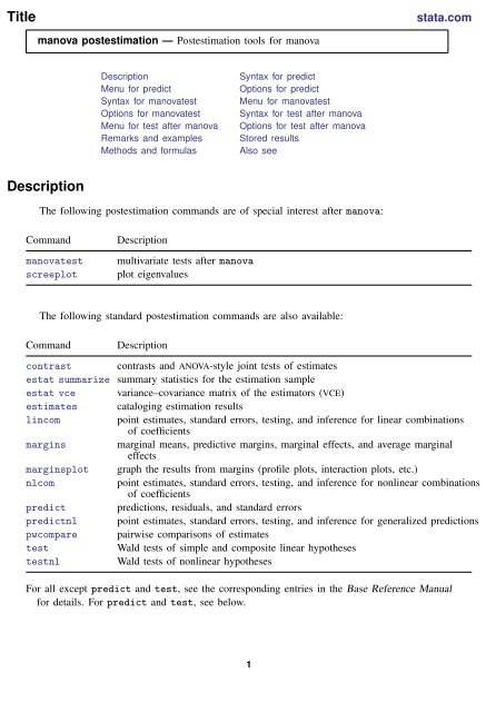
Description<br />
The following <strong>postestimation</strong> commands are of special interest after <strong>manova</strong>:<br />
Command<br />
<strong>manova</strong>test<br />
screeplot<br />
Description<br />
multivariate tests after <strong>manova</strong><br />
plot eigenvalues<br />
The following standard <strong>postestimation</strong> commands are also available:<br />
Command<br />
Description<br />
contrast contrasts and ANOVA-style joint tests of estimates<br />
estat summarize summary statistics for the estimation sample<br />
estat vce variance–covariance matrix of the estimators (VCE)<br />
estimates cataloging estimation results<br />
lincom<br />
point estimates, standard errors, testing, and inference for linear combinations<br />
of coefficients<br />
margins marginal means, predictive margins, marginal effects, and average marginal<br />
effects<br />
marginsplot graph the results from margins (profile plots, interaction plots, etc.)<br />
nlcom<br />
point estimates, standard errors, testing, and inference for nonlinear combinations<br />
of coefficients<br />
predict predictions, residuals, and standard errors<br />
predictnl point estimates, standard errors, testing, and inference for generalized predictions<br />
pwcompare pairwise comparisons of estimates<br />
test<br />
Wald tests of simple and composite linear hypotheses<br />
testnl<br />
Wald tests of nonlinear hypotheses<br />
For all except predict and test, see the corresponding entries in the Base Reference Manual<br />
for details. For predict and test, see below.<br />
1
2 <strong>manova</strong> <strong>postestimation</strong> — Postestimation tools for <strong>manova</strong><br />
Special-interest <strong>postestimation</strong> commands<br />
<strong>manova</strong>test provides multivariate tests involving terms or linear combinations of the underlying<br />
design matrix from the most recently fit <strong>manova</strong>. The four multivariate test statistics are Wilks’<br />
lambda, Pillai’s trace, Lawley–Hotelling trace, and Roy’s largest root. The format of the output is<br />
similar to that shown by <strong>manova</strong>; see [MV] <strong>manova</strong>.<br />
In addition to the standard syntax of test (see [R] test), test after <strong>manova</strong> has two additionally<br />
allowed syntaxes; see below. test performs Wald tests of expressions involving the coefficients of<br />
the underlying regression model. Simple and composite linear hypotheses are possible.<br />
Syntax for predict<br />
predict [ type ] newvar [ if ] [ in ] [ , equation(eqno [ , eqno ] ) statistic ]<br />
statistic<br />
Main<br />
xb<br />
stdp<br />
residuals<br />
difference<br />
stddp<br />
Description<br />
x j b, fitted values; the default<br />
standard error of the fitted value<br />
residuals<br />
difference between the linear predictions of two equations<br />
standard error of the fitted values for differences<br />
These statistics are available both in and out of sample; type predict . . . if e(sample) . . . if wanted only<br />
for the estimation sample.<br />
Menu for predict<br />
Statistics > Postestimation > Predictions, residuals, etc.<br />
Options for predict<br />
✄ <br />
✄ Main<br />
equation(eqno [ , eqno ] ) specifies the equation to which you are referring.<br />
equation() is filled in with one eqno for the xb, stdp, and residuals options. equation(#1)<br />
would mean that the calculation is to be made for the first equation (that is, for the first<br />
dependent variable), equation(#2) would mean the second, and so on. You could also refer to<br />
the equations by their names. equation(income) would refer to the equation named income and<br />
equation(hours), to the equation named hours.<br />
If you do not specify equation(), results are the same as if you had specified equation(#1).<br />
difference and stddp refer to between-equations concepts. To use these options, you must<br />
specify two equations, for example, equation(#1,#2) or equation(income,hours). When<br />
two equations must be specified, equation() is required. With equation(#1,#2), difference<br />
computes the prediction of equation(#1) minus the prediction of equation(#2).<br />
xb, the default, calculates the fitted values—the prediction of x j b for the specified equation.<br />
stdp calculates the standard error of the prediction for the specified equation (the standard error of<br />
the estimated expected value or mean for the observation’s covariate pattern). The standard error<br />
of the prediction is also referred to as the standard error of the fitted value.
<strong>manova</strong> <strong>postestimation</strong> — Postestimation tools for <strong>manova</strong> 3<br />
residuals calculates the residuals.<br />
difference calculates the difference between the linear predictions of two equations in the system.<br />
stddp calculates the standard error of the difference in linear predictions (x 1j b − x 2j b) between<br />
equations 1 and 2.<br />
For more information on using predict after multiple-equation estimation commands, see [R] predict.<br />
Syntax for <strong>manova</strong>test<br />
<strong>manova</strong>test term [ term . . . ] [ / term [ term . . . ] ] [ , ytransform(matname) ]<br />
<strong>manova</strong>test , test(matname) [ ytransform(matname) ]<br />
<strong>manova</strong>test , showorder<br />
where term is a term from the termlist in the previously run <strong>manova</strong>.<br />
Menu for <strong>manova</strong>test<br />
Statistics > Multivariate analysis > MANOVA, multivariate regression, and related > Multivariate tests after MANOVA<br />
Options for <strong>manova</strong>test<br />
ytransform(matname) specifies a matrix for transforming the y variables (the depvarlist from<br />
<strong>manova</strong>) as part of the test. The multivariate tests are based on (AEA ′ ) −1 (AHA ′ ). By default,<br />
A is the identity matrix. ytransform() is how you specify an A matrix to be used in the<br />
multivariate tests. Specifying ytransform() provides the same results as first transforming the<br />
y variables with YA ′ , where Y is the matrix formed by binding the y variables by column and<br />
A is the matrix stored in matname; then performing <strong>manova</strong> on the transformed y’s; and finally<br />
running <strong>manova</strong>test without ytransform().<br />
The number of columns of matname must equal the number of variables in the depvarlist from<br />
<strong>manova</strong>. The number of rows must be less than or equal to the number of variables in the depvarlist<br />
from <strong>manova</strong>. matname should have columns in the same order as the depvarlist from <strong>manova</strong>.<br />
The column and row names of matname are ignored.<br />
When ytransform() is specified, a listing of the transformations is presented before the table<br />
containing the multivariate tests. You should examine this table to verify that you have applied<br />
the transformation you desired.<br />
test(matname) is required with the second syntax of <strong>manova</strong>test. The rows of matname specify<br />
linear combinations of the underlying design matrix of the MANOVA that are to be jointly tested.<br />
The columns correspond to the underlying design matrix (including the constant if it has not been<br />
suppressed). The column and row names of matname are ignored.<br />
A listing of the constraints imposed by the test() option is presented before the table containing<br />
the multivariate tests. You should examine this table to verify that you have applied the linear<br />
combinations you desired. Typing <strong>manova</strong>test, showorder allows you to examine the ordering<br />
of the columns for the design matrix from the MANOVA.<br />
showorder causes <strong>manova</strong>test to list the definition of each column in the design matrix. showorder<br />
is not allowed with any other option or when terms are specified.
4 <strong>manova</strong> <strong>postestimation</strong> — Postestimation tools for <strong>manova</strong><br />
Syntax for test after <strong>manova</strong><br />
In addition to the standard syntax of test (see [R] test), test after <strong>manova</strong> also allows the<br />
following.<br />
test , test(matname) [ mtest [ (opt) ] matvlc(matname) ]<br />
syntax A<br />
test , showorder<br />
syntax B<br />
syntax A<br />
syntax B<br />
test expression involving the coefficients of the underlying multivariate regression<br />
model; you provide information as a matrix<br />
show underlying order of design matrix, which is useful when constructing the<br />
matname argument of the test() option<br />
Menu for test after <strong>manova</strong><br />
Statistics > Multivariate analysis > MANOVA, multivariate regression, and related > Wald test after MANOVA<br />
Options for test after <strong>manova</strong><br />
✄<br />
✄<br />
✄<br />
Main<br />
<br />
test(matname) is required with syntax A of test. The rows of matname specify linear combinations<br />
of the underlying design matrix of the MANOVA that are to be jointly tested. The columns correspond<br />
to the underlying design matrix (including the constant if it has not been suppressed). The column<br />
and row names of matname are ignored.<br />
A listing of the constraints imposed by the test() option is presented before the table containing<br />
the tests. You should examine this table to verify that you have applied the linear combinations<br />
you desired. Typing test, showorder allows you to examine the ordering of the columns for<br />
the design matrix from the MANOVA.<br />
matname should have as many columns as the number of dependent variables times the number<br />
of columns in the basic design matrix. The design matrix is repeated for each dependent variable.<br />
showorder causes test to list the definition of each column in the design matrix. showorder is<br />
not allowed with any other option.<br />
✄<br />
Options<br />
<br />
mtest [ (opt) ] specifies that tests be performed for each condition separately. opt specifies the method<br />
for adjusting p-values for multiple testing. Valid values for opt are<br />
<br />
<br />
bonferroni<br />
holm<br />
sidak<br />
noadjust<br />
Bonferroni’s method<br />
Holm’s method<br />
Šidák’s method<br />
no adjustment is to be made<br />
Specifying mtest without an argument is equivalent to specifying mtest(noadjust).
<strong>manova</strong> <strong>postestimation</strong> — Postestimation tools for <strong>manova</strong> 5<br />
The following option is available with test after <strong>manova</strong> but is not shown in the dialog box:<br />
matvlc(matname), a programmer’s option, saves the variance–covariance matrix of the linear<br />
combinations involved in the suite of tests. For the test of H 0 : Lb = c, what is returned in<br />
matname is LVL ′ , where V is the estimated variance–covariance matrix of b.<br />
Remarks and examples<br />
stata.com<br />
Several <strong>postestimation</strong> tools are available after <strong>manova</strong>. We demonstrate these tools by extending<br />
examples 1, 2, 4, and 8 of [MV] <strong>manova</strong>.<br />
Example 1: test and lincom<br />
Example 1 of [MV] <strong>manova</strong> presented a balanced one-way MANOVA on the rootstock data.<br />
. use http://www.stata-press.com/data/r13/rootstock<br />
(Table 6.2 Rootstock Data, Rencher and Christensen (2012))<br />
. <strong>manova</strong> y1 y2 y3 y4 = rootstock<br />
(output omitted )<br />
test provides Wald tests on expressions involving the underlying coefficients of the model, and<br />
lincom provides linear combinations along with standard errors and confidence intervals.<br />
. test [y3]3.rootstock = ([y3]1.rootstock + [y3]2.rootstock)/2<br />
( 1) - .5*[y3]1b.rootstock - .5*[y3]2.rootstock + [y3]3.rootstock = 0<br />
F( 1, 42) = 5.62<br />
Prob > F = 0.0224<br />
. lincom [y3]4.rootstock - [y1]4.rootstock<br />
( 1) - [y1]4.rootstock + [y3]4.rootstock = 0<br />
Coef. Std. Err. t P>|t| [95% Conf. Interval]<br />
(1) .2075001 .1443917 1.44 0.158 -.0838941 .4988943<br />
If the equation portion of the expression is omitted, the first equation (first dependent variable) is<br />
assumed.<br />
The <strong>manova</strong>test <strong>postestimation</strong> command provides multivariate tests of terms or linear combinations<br />
of the underlying design matrix from the most recent MANOVA model.<br />
Example 2: <strong>manova</strong>test<br />
In example 2 of [MV] <strong>manova</strong>, a one-way MANOVA on the metabolic dataset was shown.<br />
. use http://www.stata-press.com/data/r13/metabolic<br />
(Table 4.5 Metabolic Comparisons of Rabbits -- Rencher (1998))<br />
. <strong>manova</strong> y1 y2 = group<br />
(output omitted )<br />
<strong>manova</strong>test can test terms from the preceding <strong>manova</strong>. Here we test the group term from our<br />
one-way MANOVA:
6 <strong>manova</strong> <strong>postestimation</strong> — Postestimation tools for <strong>manova</strong><br />
. <strong>manova</strong>test group<br />
W = Wilks’ lambda<br />
P = Pillai’s trace<br />
L = Lawley-Hotelling trace<br />
R = Roy’s largest root<br />
Source Statistic df F(df1, df2) = F Prob>F<br />
group W 0.1596 3 6.0 32.0 8.02 0.0000 e<br />
P 1.2004 6.0 34.0 8.51 0.0000 a<br />
L 3.0096 6.0 30.0 7.52 0.0001 a<br />
R 1.5986 3.0 17.0 9.06 0.0008 u<br />
Residual 17<br />
e = exact, a = approximate, u = upper bound on F<br />
Using <strong>manova</strong>test to test model terms is not interesting here. It merely repeats information already<br />
presented by <strong>manova</strong>. Later we will see useful applications of term testing via <strong>manova</strong>test.<br />
<strong>manova</strong>test can also be used to test linear combinations of the underlying design matrix of the<br />
MANOVA model. Whereas the MANOVA indicates that there are differences in the groups, it does not<br />
indicate the nature of those differences. Rencher discusses three linear contrasts of interest for this<br />
example: group one (the control) versus the rest, group four versus groups two and three, and group<br />
two versus group three. The test() option of <strong>manova</strong>test allows us to test these hypotheses.<br />
Because we did not use the noconstant option with our <strong>manova</strong>, the underlying parameterization<br />
of the design matrix has the last column corresponding to the constant in the model, whereas the<br />
first four columns correspond to the four groups of rabbits. The showorder option of <strong>manova</strong>test<br />
illustrates this point. The tests on the three contrasts of interest follow.<br />
. <strong>manova</strong>test, showorder<br />
Order of columns in the design matrix<br />
1: (group==1)<br />
2: (group==2)<br />
3: (group==3)<br />
4: (group==4)<br />
5: _cons<br />
. matrix c1 = (3,-1,-1,-1,0)<br />
. <strong>manova</strong>test, test(c1)<br />
Test constraint<br />
(1) 3*1.group - 2.group - 3.group - 4.group = 0<br />
. matrix c2 = (0,-1,-1,2,0)<br />
W = Wilks’ lambda<br />
P = Pillai’s trace<br />
L = Lawley-Hotelling trace<br />
R = Roy’s largest root<br />
Source Statistic df F(df1, df2) = F Prob>F<br />
<strong>manova</strong>test W 0.4063 1 2.0 16.0 11.69 0.0007 e<br />
P 0.5937 2.0 16.0 11.69 0.0007 e<br />
L 1.4615 2.0 16.0 11.69 0.0007 e<br />
R 1.4615 2.0 16.0 11.69 0.0007 e<br />
Residual 17<br />
e = exact, a = approximate, u = upper bound on F
<strong>manova</strong> <strong>postestimation</strong> — Postestimation tools for <strong>manova</strong> 7<br />
. <strong>manova</strong>test, test(c2)<br />
Test constraint<br />
(1) - 2.group - 3.group + 2*4.group = 0<br />
. matrix c3 = (0,1,-1,0,0)<br />
. <strong>manova</strong>test, test(c3)<br />
W = Wilks’ lambda<br />
P = Pillai’s trace<br />
L = Lawley-Hotelling trace<br />
R = Roy’s largest root<br />
Source Statistic df F(df1, df2) = F Prob>F<br />
<strong>manova</strong>test W 0.9567 1 2.0 16.0 0.36 0.7018 e<br />
P 0.0433 2.0 16.0 0.36 0.7018 e<br />
L 0.0453 2.0 16.0 0.36 0.7018 e<br />
R 0.0453 2.0 16.0 0.36 0.7018 e<br />
Test constraint<br />
(1) 2.group - 3.group = 0<br />
Residual 17<br />
e = exact, a = approximate, u = upper bound on F<br />
W = Wilks’ lambda<br />
P = Pillai’s trace<br />
L = Lawley-Hotelling trace<br />
R = Roy’s largest root<br />
Source Statistic df F(df1, df2) = F Prob>F<br />
<strong>manova</strong>test W 0.4161 1 2.0 16.0 11.23 0.0009 e<br />
P 0.5839 2.0 16.0 11.23 0.0009 e<br />
L 1.4033 2.0 16.0 11.23 0.0009 e<br />
R 1.4033 2.0 16.0 11.23 0.0009 e<br />
Residual 17<br />
e = exact, a = approximate, u = upper bound on F<br />
Because there is only 1 degree of freedom for each of the hypotheses, the F tests are exact<br />
(and identical for the four multivariate methods). The first test indicates that the mean vector for the<br />
control group is significantly different from the mean vectors for the other three groups. The second<br />
test, with a p-value of 0.7018, fails to reject the null hypothesis that group four equals groups two<br />
and three. The third test, with a p-value of 0.0009, indicates differences between the mean vectors<br />
of groups two and three.<br />
Rencher also tests using weighted orthogonal contrasts. <strong>manova</strong>test can do these tests as well.<br />
. matrix c1w = (14,-7,-5,-2,0)<br />
. <strong>manova</strong>test, test(c1w)<br />
Test constraint<br />
(1) 14*1.group - 7*2.group - 5*3.group - 2*4.group = 0<br />
W = Wilks’ lambda<br />
P = Pillai’s trace<br />
L = Lawley-Hotelling trace<br />
R = Roy’s largest root<br />
Source Statistic df F(df1, df2) = F Prob>F<br />
<strong>manova</strong>test W 0.3866 1 2.0 16.0 12.70 0.0005 e<br />
P 0.6134 2.0 16.0 12.70 0.0005 e<br />
L 1.5869 2.0 16.0 12.70 0.0005 e<br />
R 1.5869 2.0 16.0 12.70 0.0005 e<br />
. matrix c2w = (0,-7,-5,12,0)<br />
Residual 17<br />
e = exact, a = approximate, u = upper bound on F
8 <strong>manova</strong> <strong>postestimation</strong> — Postestimation tools for <strong>manova</strong><br />
. <strong>manova</strong>test, test(c2w)<br />
Test constraint<br />
(1) -7*2.group - 5*3.group + 12*4.group = 0<br />
W = Wilks’ lambda<br />
P = Pillai’s trace<br />
L = Lawley-Hotelling trace<br />
R = Roy’s largest root<br />
Source Statistic df F(df1, df2) = F Prob>F<br />
<strong>manova</strong>test W 0.9810 1 2.0 16.0 0.15 0.8580 e<br />
P 0.0190 2.0 16.0 0.15 0.8580 e<br />
L 0.0193 2.0 16.0 0.15 0.8580 e<br />
R 0.0193 2.0 16.0 0.15 0.8580 e<br />
Residual 17<br />
e = exact, a = approximate, u = upper bound on F<br />
These two weighted contrasts do not lead to different conclusions compared with their unweighted<br />
counterparts.<br />
Technical note<br />
<strong>manova</strong>test, test(matname) displays the linear combination (labeled “Test constraint”) indicated<br />
by matname. You should examine this listing to make sure that the matrix you specify in test()<br />
provides the test you want.<br />
The margins <strong>postestimation</strong> command provides, among other things, tables of predicted means<br />
and confidence intervals that are based on the most recently fit model.<br />
Example 3: Margins, contrasts, and predictions<br />
Example 4 of [MV] <strong>manova</strong> presented a two-way MANOVA model on the jaw data.<br />
. use http://www.stata-press.com/data/r13/jaw<br />
(Table 4.6 Two-Way Unbalanced Data for Fractures of the Jaw -- Rencher (1998))<br />
. <strong>manova</strong> y1 y2 y3 = gender fracture gender#fracture<br />
(output omitted )<br />
The interaction term, gender#fracture, was significant. margins may be used to examine the<br />
interaction; see [R] margins.
<strong>manova</strong> <strong>postestimation</strong> — Postestimation tools for <strong>manova</strong> 9<br />
. margins gender#fracture, predict(equation(y1))<br />
Adjusted predictions Number of obs = 27<br />
Expression<br />
: Linear prediction, predict(equation(y1))<br />
Delta-method<br />
Margin Std. Err. t P>|t| [95% Conf. Interval]<br />
gender#<br />
fracture<br />
male #<br />
one compo.. 39.5 4.171386 9.47 0.000 30.82513 48.17487<br />
male #<br />
two compo.. 26.875 3.612526 7.44 0.000 19.36234 34.38766<br />
male #<br />
one simpl.. 45.16667 4.171386 10.83 0.000 36.49179 53.84154<br />
female #<br />
one compo.. 22 10.21777 2.15 0.043 .7509887 43.24901<br />
female #<br />
two compo.. 30.75 5.108884 6.02 0.000 20.12549 41.37451<br />
female #<br />
one simpl.. 36.5 7.225053 5.05 0.000 21.47468 51.52532<br />
. margins gender#fracture, predict(equation(y2))<br />
Adjusted predictions Number of obs = 27<br />
Expression<br />
: Linear prediction, predict(equation(y2))<br />
Delta-method<br />
Margin Std. Err. t P>|t| [95% Conf. Interval]<br />
gender#<br />
fracture<br />
male #<br />
one compo.. 35.5 2.150966 16.50 0.000 31.02682 39.97318<br />
male #<br />
two compo.. 32.375 1.862791 17.38 0.000 28.50111 36.24889<br />
male #<br />
one simpl.. 36.16667 2.150966 16.81 0.000 31.69349 40.63984<br />
female #<br />
one compo.. 56 5.268768 10.63 0.000 45.043 66.957<br />
female #<br />
two compo.. 33.25 2.634384 12.62 0.000 27.7715 38.7285<br />
female #<br />
one simpl.. 33 3.725582 8.86 0.000 25.25223 40.74777
10 <strong>manova</strong> <strong>postestimation</strong> — Postestimation tools for <strong>manova</strong><br />
. margins gender#fracture, predict(equation(y3))<br />
Adjusted predictions Number of obs = 27<br />
Expression<br />
: Linear prediction, predict(equation(y3))<br />
Delta-method<br />
Margin Std. Err. t P>|t| [95% Conf. Interval]<br />
gender#<br />
fracture<br />
male #<br />
one compo.. 61.16667 2.038648 30.00 0.000 56.92707 65.40627<br />
male #<br />
two compo.. 62.25 1.765521 35.26 0.000 58.5784 65.9216<br />
male #<br />
one simpl.. 58.16667 2.038648 28.53 0.000 53.92707 62.40627<br />
female #<br />
one compo.. 43 4.993647 8.61 0.000 32.61514 53.38486<br />
female #<br />
two compo.. 64 2.496823 25.63 0.000 58.80757 69.19243<br />
female #<br />
one simpl.. 63.5 3.531041 17.98 0.000 56.1568 70.8432<br />
The first margins table shows the predicted mean (marginal mean), standard error, z statistic,<br />
p-value, and confidence interval of y1 (age of patient) for each combination of fracture and gender.<br />
The second and third margins tables provide this information for y2 (blood lymphocytes) and y3<br />
(blood polymorphonuclears). These three tables of predictions are the same as those you would obtain<br />
from margins after running anova for each of the three dependent variables separately.<br />
The predicted y2 value is larger than the predicted y3 value for females with one compound<br />
fracture. For the other five combinations of gender and fracture, the relationship is reversed. There<br />
is only 1 observation for the combination of female and one compound fracture.<br />
There are nine possible contrasts if we contrast women with men for every fracture type and<br />
every dependent variable. We will use contrast to estimate all nine contrasts and apply Scheffé’s<br />
adjustment for multiple comparisons.
<strong>manova</strong> <strong>postestimation</strong> — Postestimation tools for <strong>manova</strong> 11<br />
. contrast gender@fracture#_eqns, mcompare(scheffe)<br />
Contrasts of marginal linear predictions<br />
Margins<br />
: asbalanced<br />
Scheffe<br />
df F P>F P>F<br />
gender@fracture#_eqns<br />
one compound fracture 1 1 2.51 0.1278 0.9733<br />
one compound fracture 2 1 12.98 0.0017 0.2333<br />
one compound fracture 3 1 11.34 0.0029 0.3137<br />
two compound fractures 1 1 0.38 0.5424 1.0000<br />
two compound fractures 2 1 0.07 0.7889 1.0000<br />
two compound fractures 3 1 0.33 0.5732 1.0000<br />
one simple fracture 1 1 1.08 0.3107 0.9987<br />
one simple fracture 2 1 0.54 0.4698 0.9999<br />
one simple fracture 3 1 1.71 0.2050 0.9929<br />
Joint 9 2.57 0.0361<br />
Denominator 21<br />
Note: Scheffe-adjusted p-values are reported for tests on individual<br />
contrasts only.<br />
Number of<br />
Comparisons<br />
gender@fracture#_eqns 9<br />
Scheffe<br />
Contrast Std. Err. [95% Conf. Interval]<br />
gender@fracture#_eqns<br />
(female vs base)<br />
one compound fracture 1 -17.5 11.03645 -68.42869 33.42869<br />
(female vs base)<br />
one compound fracture 2 20.5 5.69092 -5.76126 46.76126<br />
(female vs base)<br />
one compound fracture 3 -18.16667 5.393755 -43.05663 6.723297<br />
(female vs base)<br />
two compound fractures 1 3.875 6.257079 -24.99885 32.74885<br />
(female vs base)<br />
two compound fractures 2 .875 3.226449 -14.01373 15.76373<br />
(female vs base)<br />
two compound fractures 3 1.75 3.057972 -12.36128 15.86128<br />
(female vs base)<br />
one simple fracture 1 -8.666667 8.342772 -47.16513 29.8318<br />
(female vs base)<br />
one simple fracture 2 -3.166667 4.301931 -23.01831 16.68498<br />
(female vs base)<br />
one simple fracture 3 5.333333 4.077296 -13.48171 24.14838<br />
Women do not differ significantly from men in any of the nine comparisons.
12 <strong>manova</strong> <strong>postestimation</strong> — Postestimation tools for <strong>manova</strong><br />
Let’s examine the residuals with the predict command:<br />
. predict y1res, residual equation(y1)<br />
. predict y2res, residual equation(y2)<br />
. predict y3res, residual equation(y3)<br />
. list gender fracture y1res y2res y3res<br />
gender fracture y1res y2res y3res<br />
1. male one compound fracture 2.5 -.5 -.1666667<br />
2. male one compound fracture 2.5 7.5 -6.166667<br />
3. male one compound fracture 8.5 -.5 2.833333<br />
4. male one compound fracture -4.5 -2.5 3.833333<br />
5. male one compound fracture -14.5 -4.5 2.833333<br />
6. male one compound fracture 5.5 .5 -3.166667<br />
7. male two compound fractures -3.875 -5.375 1.75<br />
8. male two compound fractures -4.875 -.375 1.75<br />
9. male two compound fractures -1.875 -2.375 1.75<br />
10. male two compound fractures 1.125 6.625 -6.25<br />
11. male two compound fractures -2.875 -1.375 6.75<br />
12. male two compound fractures 25.125 -4.375 -2.25<br />
13. male two compound fractures -9.875 -2.375 1.75<br />
14. male two compound fractures -2.875 9.625 -5.25<br />
15. male one simple fracture -13.16667 .8333333 -4.166667<br />
16. male one simple fracture 6.833333 -2.166667 3.833333<br />
17. male one simple fracture 7.833333 8.833333 -7.166667<br />
18. male one simple fracture 3.833333 -1.166667 1.833333<br />
19. male one simple fracture 9.833333 -4.166667 1.833333<br />
20. male one simple fracture -15.16667 -2.166667 3.833333<br />
21. female one compound fracture 0 0 0<br />
22. female two compound fractures -8.75 -4.25 4<br />
23. female two compound fractures 7.25 -8.25 9<br />
24. female two compound fractures -9.75 3.75 -5<br />
25. female two compound fractures 11.25 8.75 -8<br />
26. female one simple fracture 6.5 -3 3.5<br />
27. female one simple fracture -6.5 3 -3.5<br />
The single observation for a female with one compound fracture has residuals that are within<br />
roundoff of zero. With only 1 observation for that cell of the design, this MANOVA model is forced<br />
to fit to that point. The largest residual (in absolute value) appears for observation 12, which has an<br />
age 25.125 higher than the model prediction for a male with two compound fractures.<br />
Example 4: <strong>manova</strong>test<br />
Example 8 of [MV] <strong>manova</strong> presents a nested MANOVA on the videotrainer data.<br />
. use http://www.stata-press.com/data/r13/videotrainer, clear<br />
(video training)<br />
. <strong>manova</strong> primary extra = video / store|video / associate|store|video /,<br />
> dropemptycells<br />
(output omitted )
<strong>manova</strong> <strong>postestimation</strong> — Postestimation tools for <strong>manova</strong> 13<br />
The MANOVA indicated that store was not significant.<br />
You decide to follow the rule of thumb that says to pool terms whose p-values are larger than<br />
0.25. Wilks’ lambda reports a p-value of 0.5775 for the test of store|video (see example 8 of<br />
[MV] <strong>manova</strong>). You decide to pool the store and associate terms in the MANOVA to gain power<br />
for the test of video. The forward-slash notation of <strong>manova</strong> is also allowed with <strong>manova</strong>test to<br />
indicate nonresidual error terms. Here is the multivariate test of video using the pooled store and<br />
associate terms and then the multivariate test of the pooled term:<br />
. <strong>manova</strong>test video / store|video associate|store|video<br />
W = Wilks’ lambda<br />
P = Pillai’s trace<br />
L = Lawley-Hotelling trace<br />
R = Roy’s largest root<br />
Source Statistic df F(df1, df2) = F Prob>F<br />
video W 0.4079 1 2.0 9.0 6.53 0.0177 e<br />
P 0.5921 2.0 9.0 6.53 0.0177 e<br />
L 1.4516 2.0 9.0 6.53 0.0177 e<br />
R 1.4516 2.0 9.0 6.53 0.0177 e<br />
store|video associate| 10<br />
store|video<br />
. <strong>manova</strong>test store|video associate|store|video<br />
e = exact, a = approximate, u = upper bound on F<br />
W = Wilks’ lambda<br />
P = Pillai’s trace<br />
L = Lawley-Hotelling trace<br />
R = Roy’s largest root<br />
Source Statistic df F(df1, df2) = F Prob>F<br />
store|video associate| W 0.3925 10 20.0 58.0 1.73 0.0546 e<br />
store|video P 0.7160 20.0 60.0 1.67 0.0647 a<br />
L 1.2711 20.0 56.0 1.78 0.0469 a<br />
R 0.9924 10.0 30.0 2.98 0.0100 u<br />
Residual 30<br />
e = exact, a = approximate, u = upper bound on F<br />
Pooling store with associate helps increase the power for the test of video.<br />
You can show the univariate analysis for one of your dependent variables by using the ytransform()<br />
option of <strong>manova</strong>test:<br />
. mat primonly = (1,0)<br />
. <strong>manova</strong>test video / store|video associate|store|video, ytransform(primonly)<br />
Transformation of the dependent variables<br />
(1) primary<br />
W = Wilks’ lambda<br />
P = Pillai’s trace<br />
L = Lawley-Hotelling trace<br />
R = Roy’s largest root<br />
Source Statistic df F(df1, df2) = F Prob>F<br />
video W 0.8449 1 1.0 10.0 1.84 0.2053 e<br />
P 0.1551 1.0 10.0 1.84 0.2053 e<br />
L 0.1835 1.0 10.0 1.84 0.2053 e<br />
R 0.1835 1.0 10.0 1.84 0.2053 e<br />
store|video associate| 10<br />
store|video<br />
e = exact, a = approximate, u = upper bound on F
14 <strong>manova</strong> <strong>postestimation</strong> — Postestimation tools for <strong>manova</strong><br />
. <strong>manova</strong>test store|video associate|store|video, ytransform(primonly)<br />
Transformation of the dependent variables<br />
(1) primary<br />
W = Wilks’ lambda<br />
P = Pillai’s trace<br />
L = Lawley-Hotelling trace<br />
R = Roy’s largest root<br />
Source Statistic df F(df1, df2) = F Prob>F<br />
store|video associate| W 0.6119 10 10.0 30.0 1.90 0.0846 e<br />
store|video P 0.3881 10.0 30.0 1.90 0.0846 e<br />
L 0.6344 10.0 30.0 1.90 0.0846 e<br />
R 0.6344 10.0 30.0 1.90 0.0846 e<br />
Residual 30<br />
e = exact, a = approximate, u = upper bound on F<br />
See the second <strong>manova</strong> run from example 8 of [MV] <strong>manova</strong> for an alternate way of pooling the<br />
terms by refitting the MANOVA model.<br />
See examples 6, 10, 11, 12, and 13 of [MV] <strong>manova</strong> for more examples of <strong>manova</strong>test, including<br />
examples involving both the test() and the ytransform() options.<br />
Stored results<br />
<strong>manova</strong>test stores the following in r():<br />
Scalars<br />
r(df)<br />
r(df r)<br />
Matrices<br />
r(H)<br />
r(E)<br />
r(stat)<br />
r(eigvals)<br />
r(aux)<br />
hypothesis degrees of freedom<br />
residual degrees of freedom<br />
hypothesis SSCP matrix<br />
residual-error SSCP matrix<br />
multivariate statistics<br />
eigenvalues of E −1 H<br />
s, m, and n values<br />
test after <strong>manova</strong> stores the following in r():<br />
Scalars<br />
r(p) two-sided p-value<br />
r(F)<br />
F statistic<br />
r(df) hypothesis degrees of freedom<br />
r(df r) residual degrees of freedom<br />
r(drop) 0 if no constraints dropped, 1 otherwise<br />
r(dropped #) index of #th constraint dropped<br />
Macros<br />
r(mtmethod)<br />
Matrices<br />
r(mtest)<br />
method of adjustment for multiple testing<br />
multiple test results<br />
Methods and formulas<br />
See [MV] <strong>manova</strong> for methods and formulas for the multivariate tests performed by <strong>manova</strong>test.
Also see<br />
[MV] <strong>manova</strong> — Multivariate analysis of variance and covariance<br />
[MV] screeplot — Scree plot<br />
[U] 20 Estimation and <strong>postestimation</strong> commands<br />
<strong>manova</strong> <strong>postestimation</strong> — Postestimation tools for <strong>manova</strong> 15


