Suitability of Correlation Arrays and Superresolution for Minehunting ...

DSTO-TN-0443
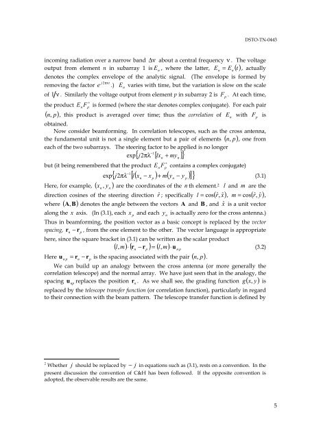
incoming radiation over a narrow band ∆ ν about a central frequency ν . The voltage
output from element n in subarray 1 is E
n
, where the latter, E = n
En
() t , actually
denotes the complex envelope of the analytic signal. (The envelope is formed by
j t
removing the factor e
2 πν .) E
n
varies with time, but the variation is slow on the scale
of 1 ν . Similarly the voltage output from element p in subarray 2 is F
p
. At each time,
∗
the product E is formed (where the star denotes complex conjugate). For each pair
n F p
( n, p)
, this product is averaged over time; thus the correlation of E n
with
F p
is
obtained.
Now consider beamforming. In correlation telescopes, such as the cross antenna,
the fundamental unit is not a single element but a pair of elements ( n, p)
, one from
each of the two subarrays. The steering factor to be applied is no longer
exp { j 2πλ −1 [ lx n
+ my n
]}
∗
but (it being remembered that the product E contains a complex conjugate)
n F p
−1
{ j2
[ l( x − x ) + m( y − y )]}
exp πλ (3.1)
n
p
Here, for example, ( x
n
, y n
) are the coordinates of the n th element. 2 l and m are the
direction cosines of the steering direction rˆ ; specifically l = cos( rˆ,
xˆ
), m = cos( rˆ,
yˆ
),
where ( A, B)
denotes the angle between the vectors A and B , and xˆ is a unit vector
along the x axis. (In (3.1), each x
p
and each y
n
is actually zero for the cross antenna.)
Thus in beamforming, the position vector as a basic concept is replaced by the vector
spacing, rn
− rp
, from the one element to the other. The vector language is appropriate
here, since the square bracket in (3.1) can be written as the scalar product
( l, m) ⋅ ( rn
− rp
) = ( l,
m) ⋅ u
n p
(3.2)
Here u
n p
= rn
− rp
is the spacing associated with the pair ( n, p)
.
We can build up an analogy between the cross antenna (or more generally the
correlation telescope) and the normal array. We have just seen that in the analogy, the
spacing u
np
replaces the position r n
. As we shall see, the grading function g ( x, y)
is
replaced by the telescope transfer function (or correlation function), particularly in regard
to their connection with the beam pattern. The telescope transfer function is defined by
n
p
2 Whether j should be replaced by j − in equations such as (3.1), rests on a convention. In the
present discussion the convention of C&H has been followed. If the opposite convention is
adopted, the observable results are the same.
5