Suitability of Correlation Arrays and Superresolution for Minehunting ...

DSTO-TN-0443
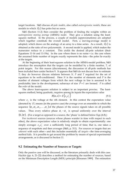
target locations. S&S discuss all-pole models, also called autoregressive models; these are
models in which ŝ () z has poles but no zeros.
S&S (Section 11-2) then consider the problem of finding the weights within an
autoregressive moving average (ARMA) model. They give a solution using the leastsquares
method. In the process, a couple of models (approximations) are adopted
which together constitute the overall model. First, a moving-average model is
adopted, which draws on the analogy of an array to a time series. As a result, ŝ () z is
obtained as the ratio of two polynomials. A second model is applied, which makes the
numerator reduce to a constant. This yields the desired all-pole solution (their
Equations 11-16 and 11-19a). In the case where there is no noise—i.e. the case where
the assumed finite number of targets exactly represents the data—the poles lie exactly
at the targets.
At the beginning of their least-squares solution to the ARMA-model problem, S&S
introduce the assumption that the targets can be modelled by a finite number, T, of
point targets. For this reason (discreteness), the discussion of all-pole methods has
been included here under Section 9. It appears that S&S do not discuss how to estimate
T; they do however discuss relations between N, P and T required for the set of
equations to be well-conditioned. Here N is the number of elements and P is the
number of element voltages from which the next voltage in line is assumed to be
predictable; later in the development, subarrays of size P + 1 are formed. P is called
the order of the model.
The above least-squares solution is subject to an important proviso. The leastsquares
method, being quadratic, requires among its inputs the expectation value
R ( m,
n ) = E { e e ∗
m n}
(9.1)
where e
n
is the voltage at the nth element. In this context the expectation value
(denoted by E ) means (in the passive case) the average over an ensemble in which the
sequence ( α
1, α
2
, α
3,
K , α s
) of the phases of the source signals takes on all possible
values. Thus every relative phase α − α is spread uniformly over the interval
( , 2π )
i
0 . (For a target as opposed to a source, the ‘phase’ is defined below Eqn (4.8).)
For incoherent sources (sources whose phases wander in time with respect to each
other), the above expectation value is relatively simple to obtain experimentally: one
∗
simply averages e me n
over a sufficiently long period of time; that is, one takes a
sequence of snapshots and then averages (S&S, p. 311). For sources or targets that are
coherent with each other—and this includes essentially all targets—the time-averaging
method fails. It is possible to get around the problem by means of special experimental
arrangements, as is discussed in Section 11.
j
9.2 Estimating the Number of Sources or Targets
Only the passive case will be discussed, as the literature primarily deals with this case.
Haykin (pp. 6, 21–22) describes a method for estimating the number of sources, based
on the Minimum Description Length (MDL) principle [Rissanen 1989]. The estimation
27