Embedding R in Windows applications, and executing R remotely
Embedding R in Windows applications, and executing R remotely
Embedding R in Windows applications, and executing R remotely

You also want an ePaper? Increase the reach of your titles
YUMPU automatically turns print PDFs into web optimized ePapers that Google loves.
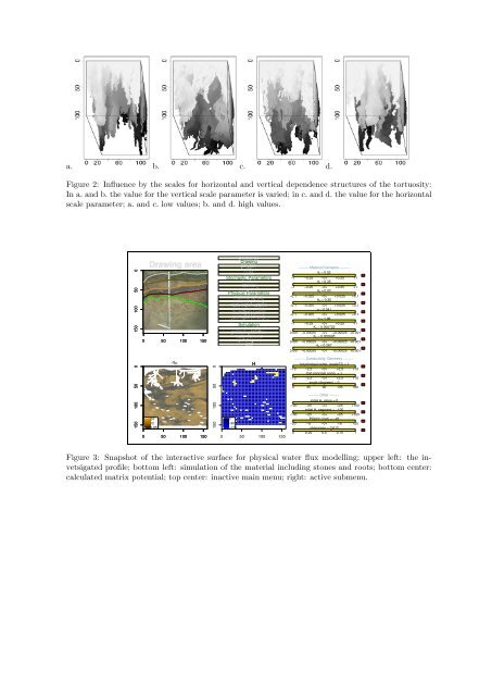
a. b. c. d.<br />
Figure 2: Influence by the scales for horizontal <strong>and</strong> vertical dependence structures of the tortuosity:<br />
In a. <strong>and</strong> b. the value for the vertical scale parameter is varied; <strong>in</strong> c. <strong>and</strong> d. the value for the horizontal<br />
scale parameter; a. <strong>and</strong> c. low values; b. <strong>and</strong> d. high values.<br />
z<br />
z<br />
150 100 50 0<br />
150 100 50 0<br />
Draw<strong>in</strong>g area<br />
postscript<br />
Draw<strong>in</strong>g<br />
polygon<br />
horizon<br />
undo<br />
Stochastic Parameters<br />
structure<br />
stones<br />
root growth<br />
Physical Parameters<br />
material (phys)<br />
material (chem)<br />
root, water uptake<br />
atmosphere, data<br />
swms2d (water)<br />
swms2d (chem)<br />
atmosphere, control<br />
Simulation<br />
new simulation<br />
precise waterflow<br />
water flow: no<br />
0 50 100 150<br />
updat<strong>in</strong>g: no<br />
end<br />
x Choose horizon or polygon!<br />
24<br />
12<br />
0.057<br />
α K<br />
z<br />
0 50 100 150<br />
150 100 50 0<br />
0<br />
−90<br />
−179<br />
H<br />
0 50 100 150<br />
−−−−− Material Constants −−−−−<br />
θ r = 0.02<br />
−1 −0.25 −0+ +0.25 +1<br />
θ s = 0.35<br />
−1 −0.25 −0+ +0.25 +1<br />
θ a = 0.02<br />
−0.1 −0.025 −0+ +0.025 +0.1<br />
θ m = 0.35<br />
−0.1 −0.025 −0+ +0.025 +0.1<br />
α = 0.041<br />
−0.1 −0.025 −0+ +0.025 +0.1<br />
n = 1.96<br />
−1 −0.25 −0+ +0.25 +1<br />
K s = 0.000722<br />
−0.001 −0.00025 −0+ +0.00025 +0.001<br />
K k = 0.000695<br />
−0.001 −0.00025 −0+ +0.00025 +0.001<br />
θ k = 0.287<br />
−0.001 −0.00025 −0+ +0.00025 +0.001<br />
−−−−− Conductivity: Geometry −−−−−<br />
1st pr<strong>in</strong>cipal comp. (scale??) = 1<br />
−10 −2.5 −0+ +2.5 +10<br />
2nd pr<strong>in</strong>cipal comp. = 1<br />
−10 −2.5 −0+ +2.5 +10<br />
angle (degrees) = 0<br />
0 45 90 135 180<br />
−−−−− Other −−−−−<br />
<strong>in</strong>itial H, slope = 0<br />
−100 −25 −0+ +25 +100<br />
<strong>in</strong>itial H, segment = −100<br />
−100 −25 −0+ +25 +100<br />
POptm (root) = −25<br />
−20 −5 −0+ +5 +20<br />
sharpness = 0.612<br />
0 0.25 0.5 0.75 1<br />
Figure 3: Snapshot of the <strong>in</strong>teractive surface for physical water flux modell<strong>in</strong>g; upper left: the <strong>in</strong>vetsigated<br />
profile; bottom left: simulation of the material <strong>in</strong>clud<strong>in</strong>g stones <strong>and</strong> roots; bottom center:<br />
calculated matrix potential; top center: <strong>in</strong>active ma<strong>in</strong> menu; right: active submenu.