Introduction to Numerical Math and Matlab ... - Ohio University
Introduction to Numerical Math and Matlab ... - Ohio University
Introduction to Numerical Math and Matlab ... - Ohio University
Create successful ePaper yourself
Turn your PDF publications into a flip-book with our unique Google optimized e-Paper software.
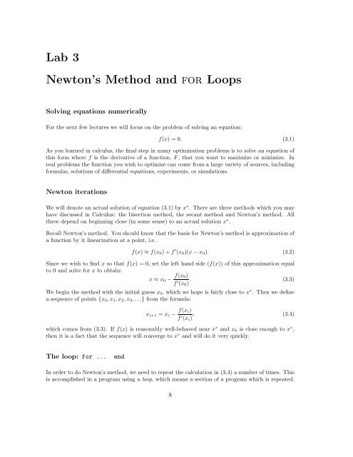
Lab 3<br />
New<strong>to</strong>n’s Method <strong>and</strong> for Loops<br />
Solving equations numerically<br />
For the next few lectures we will focus on the problem of solving an equation:<br />
f(x) = 0. (3.1)<br />
As you learned in calculus, the final step in many optimization problems is <strong>to</strong> solve an equation of<br />
this form where f is the derivative of a function, F, that you want <strong>to</strong> maximize or minimize. In<br />
real problems the function you wish <strong>to</strong> optimize can come from a large variety of sources, including<br />
formulas, solutions of differential equations, experiments, or simulations.<br />
New<strong>to</strong>n iterations<br />
We will denote an actual solution of equation (3.1) by x ∗ . There are three methods which you may<br />
have discussed in Calculus: the bisection method, the secant method <strong>and</strong> New<strong>to</strong>n’s method. All<br />
three depend on beginning close (in some sense) <strong>to</strong> an actual solution x ∗ .<br />
Recall New<strong>to</strong>n’s method. You should know that the basis for New<strong>to</strong>n’s method is approximation of<br />
a function by it linearization at a point, i.e.<br />
f(x) ≈ f(x 0 ) + f ′ (x 0 )(x − x 0 ). (3.2)<br />
Since we wish <strong>to</strong> find x so that f(x) = 0, set the left h<strong>and</strong> side (f(x)) of this approximation equal<br />
<strong>to</strong> 0 <strong>and</strong> solve for x <strong>to</strong> obtain:<br />
x ≈ x 0 − f(x 0)<br />
f ′ (x 0 ) . (3.3)<br />
We begin the method with the initial guess x 0 , which we hope is fairly close <strong>to</strong> x ∗ . Then we define<br />
a sequence of points {x 0 , x 1 , x 2 , x 3 , . . .} from the formula:<br />
x i+1 = x i − f(x i)<br />
f ′ (x i ) , (3.4)<br />
which comes from (3.3). If f(x) is reasonably well-behaved near x ∗ <strong>and</strong> x 0 is close enough <strong>to</strong> x ∗ ,<br />
then it is a fact that the sequence will converge <strong>to</strong> x ∗ <strong>and</strong> will do it very quickly.<br />
The loop: for ... end<br />
In order <strong>to</strong> do New<strong>to</strong>n’s method, we need <strong>to</strong> repeat the calculation in (3.4) a number of times. This<br />
is accomplished in a program using a loop, which means a section of a program which is repeated.<br />
8


