Introduction to Numerical Math and Matlab ... - Ohio University

Lab 9
Introduction to Linear Systems
How linear systems occur
Linear systems of equations naturally occur in many places in applications. Computers have made
it possible to quickly and accurately solve larger and larger systems of equations. Not only has this
allowed engineers and scientists to handle more and more complex problems where linear systems
naturally occur, but has also prompted engineers to use linear systems to solve problems where they
do not naturally occur such as thermodynamics, internal stress-strain analysis, fluids and chemical
processes. It has become standard practice in many areas to analyze a problem by transforming it
into a linear systems of equations and then solving those equation by computer. In this way, computers
have made linear systems of equations the most frequently used tool in modern engineering
and science.
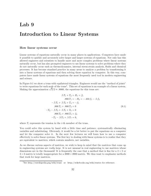
In Figure 9.1 we show a truss with equilateral triangles. Engineers would use the “method of joints”
to write equations for each node of the truss 1 . This set of equations is an example of a linear system.
Making the approximation √ 3/2 ≈ .8660, the equations for this truss are:
.5 T 1 + T 2 = R 1 = f 1
.866 T 1 = −R 2 = −.433 f 1 − .5 f 2
−.5 T 1 + .5 T 3 + T 4 = −f 1
.866 T 1 + .866 T 3 = 0
−T 2 − .5 T 3 + .5 T 5 + T 6 = 0
(9.1)
.866 T 3 + .866 T 5 = f 2
−T 4 − .5 T 5 + .5 T 7 = 0,
where T i represents the tension in the i-th member of the truss.
You could solve this system by hand with a little time and patience; systematically eliminating
variables and substituting. Obviously, it would be a lot better to put the equations on a computer
and let the computer solve it. In the next few lectures we will learn how to use a computer
effectively to solve linear systems. The first key to dealing with linear systems is to realize that they
are equivalent to matrices, which contain numbers, not variables.
As we discuss various aspects of matrices, we wish to keep in mind that the matrices that come up
in engineering systems are really large. It is not unusual in real engineering to use matrices whose
dimensions are in the thousands! It is frequently the case that a method that is fine for a 2 × 2 or
3 ×3 matrix is totally inappropriate for a 2000 ×2000 matrix. We thus want to emphasize methods
that work for large matrices.
1 See http://enwikipedia.prg/wiki/truss or http://wikebooks.org/wiki/statics for reference.
32