Introduction to Numerical Math and Matlab ... - Ohio University

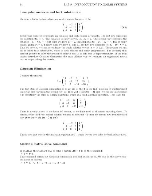
34 LAB 9. INTRODUCTION TO LINEAR SYSTEMS
Triangular matrices and back substitution
Consider a linear system whose augmented matrix happens to be:
⎛
⎝ 1 −2 3 4 ⎞
0 −1 6 7 ⎠ . (9.3)
0 0 2 4
Recall that each row represents an equation and each column a variable. The last row represents
the equation 2x 3 = 4. The equation is easily solved, i.e. x 3 = 2. The second row represents the
equation −x 2 + 6x 3 = 7, but since we know x 3 = 2, this simplifies to: −x 2 + 12 = 7. This is easily
solved, giving x 2 = 5. Finally, since we know x 2 and x 3 , the first row simplifies to: x 1 − 10 + 6 = 4.
Thus we have x 1 = 8 and so we know the whole solution vector: x = 〈8, 5, 2〉. The process we just
did is called back substitution, which is both efficient and easily programmed. The property that
made it possible to solve the system so easily is that A in this case is upper triangular. In the next
section introduce Gaussian elimination the most efficient way to transform an augmented matrix
into an upper triangular matrix.
Gaussian Elimination
Consider the matrix:
A =
⎛
⎝ 1 −2 3 4
2 −5 12 15
0 2 −10 −10
The first step of Gaussian elimination is to get rid of the 2 in the (2,1) position by subtracting 2
times the first row from the second row, i.e. (new 2nd = old 2nd - (2) 1st). We can do this because
it is essentially the same as adding equations, which is a valid algebraic operation. This leads to:
⎛
⎝ 1 −2 3 4
0 −1 6 7
0 2 −10 −10
There is already a zero in the lower left corner, so we don’t need to eliminate anything there. To
eliminate the third row, second column, we need to subtract −2 times the second row from the third
row, (new 3rd = old 3rd - (-2) 2nd):
⎛
⎝ 1 −2 3 4
0 −1 6 7
0 0 2 4
This is now just exactly the matrix in equation (9.3), which we can now solve by back substitution.
⎞
⎠ .
⎞
⎠.
⎞
⎠ .
Matlab’s matrix solve command
In Matlab the standard way to solve a system Ax = b is by the command:
> x = A\b.
This command carries out Gaussian elimination and back substitution. We can do the above computations
as follows:
> A = [1 -2 3 ; 2 -5 12 ; 0 2 -10]