Encom Discover 3D 2013 Tutorial - Pitney Bowes Software
Encom Discover 3D 2013 Tutorial - Pitney Bowes Software
Encom Discover 3D 2013 Tutorial - Pitney Bowes Software

Create successful ePaper yourself
Turn your PDF publications into a flip-book with our unique Google optimized e-Paper software.
<strong>Discover</strong> TM<br />
<strong>3D</strong> <strong>2013</strong> <strong>Tutorial</strong>s<br />
<strong>Pitney</strong> <strong>Bowes</strong> <strong>Software</strong> Inc. is a wholly-owned subsidiary of <strong>Pitney</strong> <strong>Bowes</strong> Inc. <strong>Pitney</strong> <strong>Bowes</strong>, the Corporate logo, pb<strong>Encom</strong> and <strong>Discover</strong><br />
are [registered] trademarks of <strong>Pitney</strong> <strong>Bowes</strong> Inc. or a subsidiary. All other trademarks are the property of their respective owners.<br />
© <strong>2013</strong> <strong>Pitney</strong> <strong>Bowes</strong> <strong>Software</strong> Inc. All rights reserved.
Table of Contents<br />
1 Introduction ................................................................................................ 1<br />
2 Display <strong>3D</strong> Surface and Draped Images ................................................... 5<br />
3 Drape Vectors Over Surface ................................................................... 17<br />
4 Display Point and Line Data .................................................................... 21<br />
5 Display Vector Objects in <strong>3D</strong> ................................................................... 31<br />
6 Display Drillhole Traces in <strong>3D</strong> ................................................................. 37<br />
7 Display Drillhole Sections in <strong>3D</strong> ............................................................... 49<br />
8 Create <strong>3D</strong> Object from Section Boundary ............................................... 53<br />
9 Display Downhole Logs in <strong>3D</strong> .................................................................. 57<br />
10 Display Georeferenced Image Slice ........................................................ 60<br />
11 Display Voxel Block Model in <strong>3D</strong> ............................................................. 64
Introduction 1<br />
1 Introduction<br />
This series of tutorials take you through the steps required to produce a variety<br />
of three dimensional displays with <strong>Encom</strong> <strong>Discover</strong> <strong>3D</strong>. The assorted tutorials<br />
use example data that is installed when the <strong>3D</strong> tutorial files are loaded onto<br />
your computer.<br />
The contained example data is derived from actual exploration and mine sites,<br />
providing a realistic dataset and examples of use in the three dimensional<br />
environment.<br />
Data types contained in the tutorial include:<br />
• Topographic DEM surfaces<br />
• Airphotos<br />
• Geological<br />
• Drillhole<br />
• Geophysical grids<br />
• Subsurface geophysical data<br />
• Three dimensional DXF mine development, orebody and fault plane<br />
objects<br />
• <strong>3D</strong> inversion and <strong>3D</strong> Voxel models
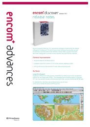
Introduction 2<br />
Example <strong>Discover</strong> <strong>3D</strong> display.<br />
<strong>Tutorial</strong> Data Installation<br />
The tutorial dataset is installed into the following locations:<br />
..\\Documents and Settings\All Users\Application<br />
Data\<strong>Encom</strong>\<strong>Discover</strong>\<strong>Discover</strong> <strong>3D</strong> <strong>Tutorial</strong> (on Windows XP operating<br />
system) or<br />
..\\ ProgramData\<strong>Encom</strong>\<strong>Discover</strong>\<strong>Discover</strong> <strong>3D</strong> <strong>Tutorial</strong> (on Windows 7 and<br />
8 operating systems)<br />
All references to the dataset locations in the tutorial exercises ignore the<br />
pathing up to <strong>Discover</strong> <strong>3D</strong> <strong>Tutorial</strong>.<br />
Within the <strong>Discover</strong> <strong>3D</strong> <strong>Tutorial</strong> folder are a series of sub-folders named to<br />
reflect the data contents.<br />
These sub-folders include:<br />
• Drilling Data – Collar, survey, assay and lithology tables.<br />
• Example Sessions and Workspaces – MapInfo Professional and<br />
<strong>Discover</strong> <strong>3D</strong> workspace and session files.<br />
• Geochem – Soil geochemistry survey files with point samples.
Introduction 3<br />
• Geology – Surface mapping data plus subsurface interpretations.<br />
• Geophysics –Magnetic <strong>3D</strong> inversion data.<br />
• Orebody Models – Orebody subsurface and surface outlines, structural<br />
fault interpretations and mine development data.<br />
• Sections –<strong>Discover</strong> drillhole sections and logs.<br />
• Topography – Elevation, topographic, airphoto and infrastructure<br />
MapInfo Professional tables.
Display <strong>3D</strong> Surface and Draped Images 5<br />
2 Display <strong>3D</strong> Surface and Draped<br />
Images<br />
This tutorial describes how to display a map created in MapInfo Professional<br />
into <strong>Discover</strong> <strong>3D</strong>.<br />
A prior level of knowledge navigating in the <strong>3D</strong> environment is required. For<br />
additional information on MapInfo Professional and <strong>Discover</strong>, refer to both the<br />
MapInfo Professional User Guide and the <strong>Discover</strong> User Guide.<br />
Step 1 – Open Workspace<br />
1. From the MapInfo Professional menu bar, choose File>Open selecting<br />
Files of Type Workspace (*.wor) from the Open dialog. Navigate to the<br />
following folder:<br />
<strong>Discover</strong> <strong>3D</strong>\<strong>Discover</strong> <strong>3D</strong> <strong>Tutorial</strong>\Example Sessions and<br />
Workspaces<br />
Open the following workspace file:<br />
<strong>Tutorial</strong> - Surface Display.WOR<br />
Step 2 – Display <strong>3D</strong> Surface<br />
Numerous methods are available for transferring data into the <strong>3D</strong> environment.<br />
2. In MapInfo Professional, navigate to <strong>Discover</strong><strong>3D</strong>>View Surface in <strong>3D</strong>.<br />
Select the Topography_RL surface file to display in <strong>3D</strong>, click OK.<br />
Transfer surface into <strong>Discover</strong> <strong>3D</strong>.
Display <strong>3D</strong> Surface and Draped Images 6<br />
Display surface in <strong>Discover</strong> <strong>3D</strong>.<br />
Step 3 – Navigate in <strong>Discover</strong> <strong>3D</strong><br />
<strong>Discover</strong> <strong>3D</strong> is divided into the following components:<br />
• Main menu<br />
• Dockable toolbars<br />
• Workspace Tree Window<br />
• <strong>3D</strong> Display Window<br />
• Information Windows<br />
• Status Bar
Display <strong>3D</strong> Surface and Draped Images 7<br />
Components of the <strong>Discover</strong> <strong>3D</strong> window.<br />
3. Two cursor control options are available for navigating or selecting view<br />
positions and movement. Navigate around the <strong>3D</strong> window using each<br />
option.<br />
4. The Select/Navigate control is used to make windows active, navigate<br />
in <strong>3D</strong>, select and edit objects and list items. Control of the <strong>3D</strong> view is<br />
based on the cursor location. It allows the <strong>3D</strong> display to spin around a<br />
horizontal axis if the cursor is moved vertically (with the left mouse<br />
button depressed); or in a circular movement around an axis into the<br />
screen when the cursor is moved horizontally.<br />
5. The <strong>3D</strong> Navigation control is used to provide greater control of <strong>3D</strong><br />
display manipulation. It is used in conjunction with the mouse cursor<br />
buttons. After clicking the Select/Navigate button, move the cursor to<br />
the <strong>3D</strong> display window or by positioning the cursor in the <strong>3D</strong> view, click<br />
the right mouse button and select the Navigate <strong>3D</strong> menu option.<br />
Sensitivity and speed of movement is controlled by the cursor’s distance<br />
from the centre point of the <strong>3D</strong> window. The following mouse button and<br />
cursor sequences allow <strong>3D</strong> navigation and flight movement:<br />
• Left mouse button depressed with vertical movement rotates the<br />
image about a horizontal axis
Display <strong>3D</strong> Surface and Draped Images 8<br />
• Left mouse button depressed with horizontal movement rotates<br />
the image about a vertical axis<br />
• Right mouse button with vertical movement zooms the image in or<br />
out of the display. Horizontal movement does nothing.<br />
• Left and Right buttons depressed with horizontal cursor<br />
movement pans the view left or right.<br />
• Left and Right buttons depressed with vertical cursor movement<br />
produces a ‘fly-through’ operation. Combining this movement with<br />
a horizontal cursor movement allows a directional fly-through of<br />
an image.<br />
Keyboard entries with mouse manipulation can also be used to control <strong>3D</strong><br />
display operation. Available combinations include:<br />
• SHIFT key plus pressed left mouse button repositions image view by<br />
panning vertically or horizontally (this only operates in <strong>3D</strong> Navigation<br />
mode). Nearing the centre of the view reduces the speed of panning.<br />
• CTRL key plus pressed left mouse button repositions image view by<br />
rotation about the horizontal and vertical axes. This can result in the<br />
image rotating as well as panning (this only operates in <strong>3D</strong> Navigation<br />
mode). With the CTRL key pressed, the <strong>3D</strong> cursor functionality moves<br />
the focus of the eye such that you can rotate the view about your current<br />
eye position. Nearing the centre of the view reduces the speed of<br />
panning.<br />
Note<br />
The numeric keys 1 -> 0 can be used to control the speed of rotation and<br />
zoom, where 1 & 2 are the slowest and 9 & 0 the fastest. This is particularly<br />
useful when navigating at high zoom through large datasets.<br />
Step 4 – Drape Geology Layer over Surface<br />
Map window data can be displayed as a draped image to provide relief and<br />
accurate representation of the surface topography.<br />
6. Within MapInfo Professional, using the Layer Control, make sure the<br />
Surface_Geology layer visible and ordered above the Topography_RL<br />
layer.<br />
7. With both tables displayed in the mapper, use either the right mouse click<br />
View in <strong>3D</strong>... or, select <strong>Discover</strong><strong>3D</strong>>View Map in <strong>3D</strong>... menu item.<br />
Specify the Surface_Geology layer to drape over the Topography_RL<br />
surface.
Display <strong>3D</strong> Surface and Draped Images 9<br />
Drape geology layer over surface topography.<br />
Note<br />
The Save Permanently option will save a copy of the draped map as an<br />
.EGB (<strong>Encom</strong> Georeferenced Bitmap) file. If this option is not selected a<br />
temporary table will be created and cannot be referenced in the future.<br />
8. To enable the display of the geology drape disable the visibility of the<br />
Surface object in the Workspace Tree.<br />
By default the white background of the geology is transparent; navigate to the<br />
Images Properties dialog by right clicking on the Images object in the<br />
Workspace Tree. Select the Image tab and uncheck the Specify transparent<br />
colour option to display the white background.
Display <strong>3D</strong> Surface and Draped Images 10<br />
Disable colour transparency.<br />
Draped geology layer on surface topography.
Display <strong>3D</strong> Surface and Draped Images 11<br />
Step 5 – Drape Air Photo over Surface<br />
The same procedure used for the surface geology can be applied to an<br />
airphoto.<br />
9. Within MapInfo Professional, using the layer control, make sure the<br />
Airphoto layer visible and ordered above the Topography_RL layer.<br />
With both tables displayed in the mapper, use either the right mouse click<br />
View in <strong>3D</strong>... or, select <strong>Discover</strong><strong>3D</strong>>View Map in <strong>3D</strong>... menu item.<br />
Specify the Airphoto layer to drape over the Topography_RL surface.<br />
To enable the display of the airphoto drape disable the visibility of the<br />
Surface object and geology drape Images object in the Workspace<br />
Tree.<br />
Navigate to the Images Properties dialog by right mouse clicking on the<br />
Images object in the Workspace Tree. Select the Transparency tab and<br />
move the Transparency slider to 30%. This will alter the display to<br />
provide the drape airphoto with a transparency.<br />
Airphoto draped over the surface topography.
Display <strong>3D</strong> Surface and Draped Images 12<br />
Step 6 – Offset layers in <strong>3D</strong><br />
From the previous exercises three objects are present in the <strong>3D</strong> Display<br />
Window, as they were derived from the same surface layer all layers are<br />
overlapping. To display all objects it may be necessary to display the layers with<br />
an offset.<br />
10. Navigate to the Images Properties dialog for the airphoto drape by right<br />
mouse clicking on the Images object in the Workspace Tree. Select the<br />
Transform tab, enter an Offset Z value of 50.<br />
11. Navigate to the Surface Properties dialog by right mouse clicking on the<br />
Surface object in the Workspace Tree. Select the Surface layer, enter<br />
an Offset value of -50.<br />
Specify offset value for surface layer.
Display <strong>3D</strong> Surface and Draped Images 13<br />
Surface layers offset in <strong>3D</strong>.<br />
Step 7 – Modify Vertical Scale<br />
12. To control the map vertical scaling navigate to the Scale tab of the <strong>3D</strong><br />
Map branch properties dialog. The slider associated with the Z Scale<br />
controls the vertical exaggeration. Set a Z scale of 2; note the scaling is<br />
applied to all datasets within the <strong>3D</strong> view.
Display <strong>3D</strong> Surface and Draped Images 14<br />
<strong>3D</strong> Map Properties dialog controlling vertical exaggeration.<br />
Surface layers offset and rescaled in <strong>3D</strong>.
Display <strong>3D</strong> Surface and Draped Images 15<br />
Note<br />
In most cases, when using the properties dialogs for modifying display<br />
controls, you will need to click the Apply button at the base of the dialog<br />
before any re-display of the view takes place.<br />
Under certain tabs an Auto Apply option is available that allows the screen<br />
view to update as changes are made in the Properties dialog.<br />
13. Complete this step of the tutorial by closing all layers in the <strong>Discover</strong> <strong>3D</strong><br />
display using the File>Close All menu item. Close all open tables in<br />
MapInfo Professional using File>Close All.
Drape Vectors Over Surface 17<br />
3 Drape Vectors Over Surface<br />
This tutorial details steps required to drape vector layers over an elevation<br />
surface.<br />
A prior level of knowledge navigating in the <strong>3D</strong> environment is required. For<br />
additional information on MapInfo Professional and <strong>Discover</strong>, refer to both the<br />
MapInfo Professional User Guide and the <strong>Discover</strong> User Guide.<br />
Step 1 – Open Workspace<br />
1. From the MapInfo Professional menu bar, choose File>Open selecting<br />
Files of Type Workspace (*.wor) from the Open dialog. Navigate to the<br />
following folder:<br />
<strong>Discover</strong> <strong>3D</strong>\<strong>Discover</strong> <strong>3D</strong> <strong>Tutorial</strong>\Example Sessions and<br />
Workspaces<br />
Open the following workspace file:<br />
<strong>Tutorial</strong> - Drape Vectors.WOR<br />
Step 2 – Display Draped Airphoto in <strong>3D</strong><br />
2. Navigate to <strong>Discover</strong><strong>3D</strong>>View Map in <strong>3D</strong>..., from the View Map in <strong>3D</strong><br />
dialog select the mapper to view and the Grid file Topography_RL as<br />
the draping surface.
Drape Vectors Over Surface 18<br />
Drape airphoto in <strong>3D</strong>.<br />
Airphoto draped over topographic surface.
Drape Vectors Over Surface 19<br />
3. Navigate back to MapInfo Professional and make the vector layers visible<br />
using layer control.<br />
Vector layer to make visible include:<br />
Roads<br />
Fences<br />
Streams<br />
Navigate to <strong>Discover</strong><strong>3D</strong>>View Objects in <strong>3D</strong>... menu. On the View<br />
objects in <strong>3D</strong> dialog select the Roads, Fences and Streams tables and<br />
Assign a Z value from the grid Topography_RL. This will create<br />
separate vector objects in <strong>3D</strong> which are draped over the selected<br />
surface.<br />
View objects in <strong>3D</strong> vector drape.
Drape Vectors Over Surface 20<br />
Vector objects draped in <strong>3D</strong> window.<br />
4. If the vector layers are located below the draped airphoto, right click on<br />
the Images branch and move to the top of the Workspace Tree or left<br />
mouse click and hold on the object and drag to the appropriate location in<br />
the Workspace Tree.<br />
Alternatively, navigate to the Images Properties dialog for the airphoto<br />
drape by right mouse clicking on the Images object in the Workspace<br />
Tree. Select the Transform tab, enter an Offset Z value of -1<br />
Within <strong>Discover</strong> <strong>3D</strong>, you can toggle the display of the vectors from the<br />
Workspace Tree by simply unchecking the vectors you wish not to view.<br />
5. If the vector lines are not thick enough access the properties of the vector<br />
layers and modify the line style from within the Surface tab.<br />
6. Complete this step of the tutorial by closing all layers in the <strong>Discover</strong> <strong>3D</strong><br />
display using the File>Close All menu item. Close all open tables in<br />
MapInfo Professional using File>Close All.
Display Point and Line Data 21<br />
4 Display Point and Line Data<br />
This tutorial describes how to display geochemical point data and modify colour<br />
based on element values in <strong>Discover</strong> <strong>3D</strong>.<br />
A prior level of knowledge navigating in the <strong>3D</strong> environment is required. For<br />
additional information on MapInfo Professional and <strong>Discover</strong>, refer to both the<br />
MapInfo Professional User Guide and the <strong>Discover</strong> User Guide.<br />
Step 1 – Open Workspace<br />
1. From the MapInfo Professional menu bar, choose File>Open selecting<br />
Files of Type Workspace (*.wor) from the Open dialog. Navigate to the<br />
following folder:<br />
<strong>Discover</strong> <strong>3D</strong>\<strong>Discover</strong> <strong>3D</strong> <strong>Tutorial</strong>\Example Sessions and<br />
Workspaces<br />
Open the following workspace file:<br />
<strong>Tutorial</strong> - Line Data Display.WOR<br />
Note<br />
The coverage of the geochemical survey extends beyond the air photo.<br />
Soil geochemical points displayed over the airphoto.
Display Point and Line Data 22<br />
Step 2 – Display Geochemical Dataset in <strong>3D</strong><br />
2. Display the Airphoto image draped over the Topography_RL surface<br />
into the <strong>3D</strong> display, navigate to <strong>Discover</strong><strong>3D</strong>><strong>3D</strong> Utilities>Overlay<br />
Image on Grid.... This will create an EGB file called Airphoto.egb, drop<br />
and drag this file into the <strong>3D</strong> Display Window from the \<strong>Discover</strong> <strong>3D</strong><br />
<strong>Tutorial</strong> \Topography folder. Open the <strong>3D</strong> Window by navigating to<br />
<strong>Discover</strong><strong>3D</strong>>Open <strong>3D</strong> Window.<br />
Note<br />
Displaying an image draped over a surface with Overlay Image on Grid tool<br />
will maintain the full image quality.<br />
3. To create <strong>3D</strong> lines navigate to <strong>Discover</strong><strong>3D</strong>>Create <strong>3D</strong> Lines... to view in<br />
<strong>3D</strong>. Alternatively to view <strong>3D</strong> points navigate to <strong>Discover</strong><strong>3D</strong>>Create <strong>3D</strong><br />
Points... option. The only difference in the <strong>3D</strong> view is the <strong>3D</strong> points<br />
option displays the individual sample points as symbols in <strong>Discover</strong> <strong>3D</strong>,<br />
whereas the <strong>3D</strong> Lines option joins the sample points as discrete lines.<br />
Create <strong>3D</strong> Lines and select the Soil_Geochemistry table to display from<br />
the Show <strong>3D</strong> Lines dialog.<br />
Select table to create line data.<br />
4. All point data will be imported as lines into the <strong>3D</strong> display. Several<br />
regional data points should be removed from the display to reduce the<br />
visual clutter. To remove lines, right mouse click the Lines item from the<br />
Workspace Tree and select Properties. Navigate to the Lines tab, and<br />
ensure all lines prefixed with Regional Line are moved to the Hide pane<br />
for the Line Selection. Click Apply to commit the change, <strong>Discover</strong> <strong>3D</strong><br />
view updates to include only the survey coverage in the vicinity of the<br />
airphoto.
Display Point and Line Data 23<br />
Remove the regional lines using the Lines Properties dialog.<br />
Step 3 – Modifying Line Appearance<br />
Numerous options are present to control the appearance of lines and point data;<br />
including style, colour and thickness.<br />
5. Display the Properties dialog of the Lines branch of the Workspace<br />
Tree and select the Appearance tab. Click the Line Style button; the<br />
dialog presented will allow modification of the line thickness, select<br />
weight of 3.5. Click the Apply button to update the display.
Display Point and Line Data 24<br />
Modify Line thickness.<br />
6. Within the survey area, copper is of significant interest. To modulate the<br />
line colour based on copper values, navigate to the Colour tab on the<br />
Lines Properties dialog, enable the Colour option. From the pull-down<br />
list, select Cu. Click the Apply button to display a colour modulated line<br />
based on copper values.<br />
7. Further colour enhancement can be performed using the colour<br />
modulation table accessed via the Edit colour scale button. The data<br />
lines reflect the changing copper values along the sampled lines.
Display Point and Line Data 25<br />
Modulate line colour based on Cu values.<br />
Step 4 – View Points from Line Data<br />
8. To view point data associated with the linework navigate to<br />
Display>Points to create a new Point object in the Workspace Tree.<br />
Display the properties dialog for the Points object (double click, or right<br />
mouse click and select Properties from the menu). From the Lines tab<br />
show all lines excluding those with a Regional Line prefix.<br />
9. Select the symbology to use from the Symbol tab. Uncheck the Fast<br />
Symbol option and select symbol type to view.<br />
Note<br />
Fast Symbols are best when viewing large amounts of data, as they require<br />
little processing memory to display.<br />
The size of the points can be modulated based on a size value. Check<br />
the Size option and specify the data field, Cu. The size of symbols can<br />
range between a minimum to maximum that can be defined and these<br />
values are used to scale the data range for sizing determined by the<br />
copper data values. Set this range between 3 and 15.
Display Point and Line Data 26<br />
Modulate point size by Cu value.<br />
Step 5 – Colour Modulate Points<br />
10. To highlight copper values colour modulate the points based on copper<br />
values. Navigate to the Colour tab and enable the Colour option. From<br />
the pull-down list, select Cu. Click the Apply button to display a colour<br />
modulated line based on copper vales.<br />
11. Further colour enhancement can be performed using the colour<br />
modulation table accessed via the Edit colour scale button. The points<br />
reflect the changing copper values along the sampled lines.
Display Point and Line Data 27<br />
Modulate points by Cu colour.<br />
Step 6 – Offset Point and Line Data<br />
Geochemical trends can be observed in the point and line datasets with<br />
modulated colour vales, however, it can be difficult to observe when obscured<br />
by the air photo. To overcome, the individual data lines and points can be offset<br />
to highlight the value ranges clearly.<br />
12. Navigate to the Fields tab on the Lines Properties dialog. Activate the<br />
Offset option and select the Cu data field from the pull-down list. Click<br />
the Apply button to offset the lines.<br />
Note<br />
Observe how the lines move up and down depending on the copper data<br />
value.<br />
13. Repeat this procedure on the Points Properties dialog, activate the<br />
Offset option and select the Cu data field from the pull-down list. For<br />
each point, the copper value is added to the Z or elevation and<br />
repositioned accordingly.
Display Point and Line Data 28<br />
Modulate point elevation by CU value.<br />
Step 7 – Display Point Information<br />
Within the <strong>3D</strong> interface information can be dynamically displayed for individual<br />
objects.<br />
14. From the Workspace Tree make the Points object selectable by<br />
activating the Select control.<br />
From the Workspace Tree make the Points object browsable by<br />
activating the Browse control.<br />
Ensure the Select/Navigate control is activated.<br />
Ensure the Data Window is open and display in <strong>3D</strong> by enabling this<br />
control from the Main toolbar.<br />
15. Slowly mouse the mouse cursor over point objects in the <strong>3D</strong> Display<br />
Window, when the mouse hovers over a point, information about that<br />
point is displayed in the Data Window.<br />
The Data Window fields can be customised by right mouse clicking in<br />
the Data Window and selecting Customise.
Display Point and Line Data 29<br />
16. Complete this step of the tutorial by closing all layers in the <strong>Discover</strong> <strong>3D</strong><br />
display using the File>Close All menu item. Close all open tables in<br />
MapInfo Professional using File>Close All.
Display Vector Objects in <strong>3D</strong> 31<br />
5 Display Vector Objects in <strong>3D</strong><br />
This tutorial shows you how to add various <strong>3D</strong> objects into the <strong>3D</strong> display.<br />
Typically, objects are created in third-party software such as modelling<br />
programs, mine planning packages or systems capable of producing <strong>3D</strong> output.<br />
A prior level of knowledge navigating in the MapInfo Professional and <strong>Discover</strong><br />
<strong>3D</strong> environment is assumed. For additional information on MapInfo Professional<br />
and <strong>Discover</strong>, refer to both the MapInfo Professional User Guide and the<br />
<strong>Discover</strong> User Guide.<br />
Step 1 – Open Dataset<br />
1. From the MapInfo Professional menu bar, choose File>Open selecting<br />
Files of Type Workspace (*.wor) from the Open dialog. Navigate to the<br />
following folder:<br />
<strong>Discover</strong> <strong>3D</strong>\<strong>Discover</strong> <strong>3D</strong> <strong>Tutorial</strong>\Example Sessions and<br />
Workspaces<br />
Open the following workspace file:<br />
<strong>Tutorial</strong> - Display DXF Vectors.WOR<br />
Orebody outline displayed on airphoto.
Display Vector Objects in <strong>3D</strong> 32<br />
Step 2 – Display Draped Map in <strong>3D</strong><br />
2. Navigate to <strong>Discover</strong> <strong>3D</strong>>View Map in <strong>3D</strong>..., from the View Map in <strong>3D</strong><br />
dialog select the mapper to view and the Grid file Topography_RL as<br />
the draping surface.<br />
Step 3 – Load DXF in <strong>3D</strong><br />
The most common and versatile <strong>3D</strong> data format is the AutoCad DXF <strong>3D</strong> format<br />
file. This file type is supported by <strong>Discover</strong> <strong>3D</strong>, in some cases and where<br />
appropriate the DXF format files can also be displayed in MapInfo Professional<br />
and <strong>Discover</strong>.<br />
3. Two methods are available to import a DXF file directly into <strong>Discover</strong> <strong>3D</strong>.<br />
Select the Display><strong>3D</strong> Vector item from the main menu or<br />
Drop-and-Drag the DXF file into <strong>Discover</strong> <strong>3D</strong> from Windows Explorer.<br />
4. Create a new <strong>3D</strong> Vector object using Display><strong>3D</strong> Vector option. Right<br />
mouse click the Vectors item from the Workspace Tree and select<br />
Properties. Navigate to the File tab, use the Browse button to specify a<br />
<strong>3D</strong> DXF file. Navigate to the Orebody Models folder and select the<br />
Skarn_Orebody.DXF file.<br />
Click the Apply button after selection to display the orebody.
Display Vector Objects in <strong>3D</strong> 33<br />
Skarn orebody displayed in <strong>3D</strong>.<br />
Step 4 – Modify DXF Appearance<br />
<strong>Discover</strong> <strong>3D</strong> provides a number of controls to modify the appearance of<br />
displayed DXF files. These controls are located on the Vector Properties dialog.<br />
5. Modify the DXF appearance by adjusting the various property controls<br />
• The geometry of the shape can be smoothed by checking the<br />
Smooth Surface option on the File tab.<br />
• The native fill colour of the object can be overridden by modifying<br />
the Fill Colour on the Surface tab.<br />
• The vertices of the DXF object can be joined by a wireframe to<br />
assist in viewing the smoothness of the object. Check the<br />
Wireframe option on the Surface tab to enable.<br />
• The transparency of the object can be altered to permit other items<br />
such as drillholes of other <strong>3D</strong> objects to become visible. On the<br />
Transparency tab move the slider to the desired transparency<br />
level.
Display Vector Objects in <strong>3D</strong> 34<br />
• To prevent self see through of a transparent object check the<br />
Prevent seeing an object through itself option on the<br />
Transparency tab.<br />
Modified DXF orebody object.<br />
Step 5 – Display Additional DXF Objects<br />
6. Navigate to the following folder:<br />
<strong>Discover</strong> <strong>3D</strong>\<strong>Discover</strong> <strong>3D</strong> <strong>Tutorial</strong>\Orebody Models<br />
From Windows Explorer Drop-and-Drag the following DXF files into the<br />
<strong>3D</strong> Display Window:<br />
Shaft.DXF<br />
Fault_1.DXF<br />
Development.DXF
Display Vector Objects in <strong>3D</strong> 35<br />
<strong>3D</strong> DXF files displayed in <strong>Discover</strong> <strong>3D</strong>.<br />
7. Complete this step of the tutorial by closing all layers in the <strong>Discover</strong> <strong>3D</strong><br />
display using the File>Close All menu item. Close all open tables in<br />
MapInfo Professional using File>Close All.
Display Drillhole Traces in <strong>3D</strong> 37<br />
6 Display Drillhole Traces in <strong>3D</strong><br />
This tutorial demonstrates the ability of <strong>Discover</strong> <strong>3D</strong> to visualise and interrogate<br />
drillhole data in three dimensions. This has obvious and significant advantages<br />
over simply viewing maps and data sections.<br />
A prior level of knowledge navigating in the <strong>3D</strong> environment is required. For<br />
additional information on how to create, import and display drillhole data, refer<br />
to the Drillhole Display section of the <strong>Discover</strong> User Guide. For additional<br />
information on MapInfo Professional and <strong>Discover</strong>, refer to both the MapInfo<br />
Professional User Guide and the <strong>Discover</strong> User Guide.<br />
Step 1 – Open <strong>3D</strong> Dataset<br />
1. From the <strong>Discover</strong> <strong>3D</strong> menu in MapInfo Professional navigate to<br />
<strong>Discover</strong><strong>3D</strong>>Open <strong>3D</strong> Window. Select the File>Open Session... menu<br />
item and navigate to the following folder:<br />
<strong>Discover</strong> <strong>3D</strong>\<strong>Discover</strong> <strong>3D</strong> <strong>Tutorial</strong>\Example Sessions and<br />
Workspaces<br />
Open the following session file:<br />
<strong>Tutorial</strong> - Drillhole Surface Drape.EGS<br />
Step 2 – Import Drillhole Project<br />
2. Navigate to the Drillhole menu item in <strong>Discover</strong> to open a supplementary<br />
Drillholes menu. Select Drillholes>Project Manager>Import/Export.<br />
Navigate to the following folder:<br />
<strong>Discover</strong> <strong>3D</strong>\<strong>Discover</strong> <strong>3D</strong> <strong>Tutorial</strong>\Drilling Data\Drillhole Project<br />
Import the following drillhole project file:<br />
Example Drilling.setup.xml<br />
When prompted by <strong>Discover</strong> import the project and accept the default<br />
name Example Drilling. Click OK.
Display Drillhole Traces in <strong>3D</strong> 38<br />
Import <strong>Discover</strong> Drillhole Project.<br />
From Drillholes menu navigate to Drillholes>Project Manager... and<br />
select the Example Drilling project. Click Open.<br />
Open <strong>Discover</strong> Drillhole Project.<br />
A mapper window containing the Drillhole_Collar table and<br />
TOPOGRAPHY_RL grid will open with the project. The other required<br />
project tables Drillhole_LITH, Drillhole_SURVEYS, Drillhole_ASSAYS<br />
will open in the background.
Display Drillhole Traces in <strong>3D</strong> 39<br />
Step 3 – Display Drillhole Traces in <strong>3D</strong><br />
3. Navigate to the <strong>Discover</strong><strong>3D</strong>>View Drillholes... option. Select all the<br />
drillholes by clicking the Select All button on the <strong>3D</strong> Drillhole Wizard<br />
dialog.<br />
Import drillholes into <strong>Discover</strong> <strong>3D</strong>.<br />
Note<br />
For very large datasets or for lower-end computers, it is advisable to import<br />
only a subset of the drillhole dataset into the <strong>3D</strong> window. To do this, tick the<br />
Load Subset based on selected option at the bottom of the dialog, ensure<br />
that only the drillholes to be imported are listed under the Selected column.<br />
Initially, drillhole traces are displayed as grey <strong>3D</strong> tubes. The collar<br />
positions of the drillholes coincide with the topographic surface that has<br />
the Airphoto draped over it.
Display Drillhole Traces in <strong>3D</strong> 40<br />
Drillhole traces displayed in <strong>Discover</strong> <strong>3D</strong>.<br />
Step 4 - Selecting Drillholes in <strong>Discover</strong> <strong>3D</strong><br />
4. Right mouse click on the Drillholes object on the Workspace Tree<br />
and select the Properties option. Navigate to the Holes tab, click the<br />
Drillhole Selection button.<br />
From the Drillhole Selection dialog use the Selection Tools to select<br />
a subset of the drillholes to display in <strong>3D</strong>. Click Apply, only the<br />
selected holes will be displayed.
Display Drillhole Traces in <strong>3D</strong> 41<br />
Subset drillholes from the Drillhole Selection dialog.<br />
Step 5 - Modify Drillhole Appearance<br />
5. From the Drillholes Properties dialog navigate to the Appearance tab.<br />
Three options are available for trace style:<br />
Line<br />
<strong>3D</strong> Tube<br />
<strong>3D</strong> Rose<br />
When large numbers of drillholes are displayed, the Line format is<br />
advisable for rapid <strong>3D</strong> display. Both the <strong>3D</strong> Tube and <strong>3D</strong> Rose option<br />
allows more comprehensive <strong>3D</strong> displays.<br />
Select the <strong>3D</strong> Tube option and increase the Thickness value to 3.
Display Drillhole Traces in <strong>3D</strong> 42<br />
Appearance tab for modulating trace style.<br />
6. To assist with visual interpretation it may be necessary to display drillhole<br />
collars and end of holes labels. This is especially useful when a surface<br />
(such as an airphoto) is draped over the collar positions. Enable the<br />
Collar Label, Bottom Label and Collar Symbol options and configure<br />
as required on the Symbols tab.
Display Drillhole Traces in <strong>3D</strong> 43<br />
Modify Drillhole labels and symbols.<br />
Step 6 - Modulate Drillhole Thickness<br />
7. Navigate to the Appearance tab and select <strong>3D</strong> Rose drillhole style. The<br />
Petals button controls the display thickness of the drill trace based on<br />
selected downhole attributes such as assay values. Select this option to<br />
display the Petal Channels dialog. The colour, size and data fields<br />
displayed are controlled from this dialog.<br />
The Petal Channels dialog controls the tube thickness of drillholes as<br />
either discs or enlarged tubes. Check the Show box to activate a field to<br />
display, specify a Field to control the drillhole diameter. Select the<br />
Drillhole_ASSAYS_AU_AVG from the Field pull-down list. Ensure both<br />
the Enhance and Global options are checked to modulate the thickness.<br />
Click the Apply button, note how the displayed drillhole diameters alter.<br />
Multiple data channels can be selected to control thickness with multiple<br />
drillhole diameters relative to the data channels selected. Experiment with<br />
modulation of the drillhole traces using multiple assay fields.
Display Drillhole Traces in <strong>3D</strong> 44<br />
Modulate trace thickness by assay value.
Display Drillhole Traces in <strong>3D</strong> 45<br />
Modulated drillhole thickness by Drillhole_ASSAYS_CU and<br />
Drillhole_ASSAY_AU_AVG.<br />
Note<br />
Performance degradation may be experienced when visualising drill traces<br />
as <strong>3D</strong> Rose Petals. For faster navigation speed use either <strong>3D</strong> Tube or Line<br />
trace styles.<br />
Step 7 - Modulate Drillhole Colour<br />
8. Ensure the drill trace is thickness modulated only by the<br />
Drillhole_ASSAYS_AU_AVG field. Navigate to the Colour tab and<br />
check the Colour box. This feature allows the colour of the drillholes to<br />
change depending on values contained within a data field. For example,<br />
drillhole assays or lithology can be used to alter not only the colour, but<br />
also the patterns of display of the drillholes.<br />
9. Select the Drillhole_ASSAYS_AU_AVG from the pull-down list. To<br />
select a specific colour scheme or legend to colour or attribute the<br />
drillhole traces, click the Apply button.
Display Drillhole Traces in <strong>3D</strong> 46<br />
The colour applied to the drill traces is relatively uniform; this is due to<br />
the presence of null assay values expressed as -1 value. To display a<br />
colour scheme which reflects the data better select the Edit Colour<br />
Mapping button. Check the Apply bandpass cutoff box and type in a<br />
lower and upper value of 5% and 95% respectively. Click OK to<br />
commit the change.<br />
Colour Mapping with cut-off applied to upper and lower data values.
Display Drillhole Traces in <strong>3D</strong> 47<br />
Modulated drillhole thicknesses by thickness and colour.<br />
Extensive control is provided over the selection and appearance of the available<br />
look-up tables and legends that provide colours or patterns to the drillholes,<br />
custom LUT tables and legends can be constructed. A range of look-up tables<br />
are supplied with <strong>Discover</strong> <strong>3D</strong> as well as a powerful Colour Lookup Editor (refer<br />
to the <strong>Discover</strong> <strong>3D</strong> User Guide).<br />
Look-up tables control the colours used in modulating the drillhole data, in<br />
addition, patterns can be used instead. Patterns use available Legends also<br />
supplied with the software, or you can use the Legend Editor to create and edit<br />
these (refer to the Legend Editor in the <strong>Discover</strong> <strong>3D</strong> User Guide).<br />
10. Complete this step of the tutorial by closing all layers in the <strong>Discover</strong> <strong>3D</strong><br />
display using the File>Close All menu item. Close all open tables in<br />
MapInfo Professional using File>Close All.
Display Drillhole Traces in <strong>3D</strong> 48<br />
Example drill trace modulation.<br />
Drill trace modulated by lithology.
Display Drillhole Sections in <strong>3D</strong> 49<br />
7 Display Drillhole Sections in <strong>3D</strong><br />
This tutorial illustrates how interpreted drillhole sections can be displayed in a<br />
<strong>3D</strong> view with the associated drillhole information. From drillhole data, logs, rock<br />
type or assay data interpretations can be created within <strong>Discover</strong> <strong>3D</strong>. When<br />
these interpretations are displayed in three dimensions their relationships can<br />
become significantly more meaningful.<br />
A prior level of knowledge navigating in the <strong>3D</strong> environment is required. For<br />
additional information on how to create, import and display drillhole data, refer<br />
to the Drillhole Display section of the <strong>Discover</strong> User Guide. For additional<br />
information on MapInfo Professional and <strong>Discover</strong>, refer to both the MapInfo<br />
Professional User Guide and the <strong>Discover</strong> User Guide.<br />
Step 1 – Open <strong>3D</strong> Dataset<br />
1. From the <strong>Discover</strong> <strong>3D</strong> menu in MapInfo Professional navigate to<br />
<strong>Discover</strong><strong>3D</strong>>Open <strong>3D</strong> Window. Select the File>Open Session... menu<br />
item and navigate to the following folder:<br />
<strong>Discover</strong> <strong>3D</strong>\<strong>Discover</strong> <strong>3D</strong> <strong>Tutorial</strong>\Example Sessions and<br />
Workspaces<br />
Open the following session file:<br />
<strong>Tutorial</strong> - Drillhole Section Display.EGS<br />
Step 2 – Open <strong>Discover</strong> Drillhole Project<br />
2. From the MapInfo Professional menu bar, navigate to<br />
<strong>Discover</strong>>Drillholes>Project Manager.... From the Project Manager<br />
select the project Example Drilling to open. If this project is not visible<br />
you will need to import as described in the Display Drillhole Traces in <strong>3D</strong><br />
tutorial.<br />
3. Navigate to Drillholes>Section Manager... and open the three<br />
previously created sections; Section_1, Section_2 and Section_3. From<br />
the Section Manager dialog, select all three available sections and then<br />
click the Open button. The digitized polygon represents a lithology layer<br />
consisting of a Lava unit.
Display Drillhole Sections in <strong>3D</strong> 50<br />
Display drillhole sections in MapInfo.<br />
Step 3 – Display Sections in <strong>3D</strong><br />
4. Navigate to <strong>Discover</strong><strong>3D</strong>>View Sections... to export the open section<br />
into <strong>3D</strong>. Highlight all three sections on the Export located bitmap dialog<br />
and click OK. Ensure only the sections are highlighted since other<br />
windows such as the collar map are inappropriate to display as sections.<br />
Export Drillhole sections to <strong>Discover</strong> <strong>3D</strong>.
Display Drillhole Sections in <strong>3D</strong> 51<br />
Drillholes sections display in <strong>Discover</strong> <strong>3D</strong>.<br />
5. Complete this step of the tutorial by closing all layers in the <strong>Discover</strong> <strong>3D</strong><br />
display using the File>Close All menu item. Close all open tables in<br />
MapInfo Professional using File>Close All.
Create <strong>3D</strong> Object from Section Boundary 53<br />
8 Create <strong>3D</strong> Object from Section<br />
Boundary<br />
This tutorial illustrates how to create a <strong>3D</strong> solid object from a series of digitized<br />
drillhole section boundary layers.<br />
A prior level of knowledge navigating in the MapInfo Professional and <strong>Discover</strong><br />
<strong>3D</strong> environment is assumed. For additional information on MapInfo Professional<br />
and <strong>Discover</strong>, refer to both the MapInfo Professional User Guide and the<br />
<strong>Discover</strong> User Guide.<br />
What are Feature Objects and Feature Database?<br />
The feature database provides a powerful utility for the creation and storage of<br />
<strong>3D</strong> Feature Objects. Feature Objects are points, lines or polygonal regions that<br />
represent entities such as geological/ore boundaries, structural/fault<br />
intersections or other general features of interest in the <strong>3D</strong> environment. These<br />
objects can be created in <strong>Discover</strong><strong>3D</strong>, exported from MapInfo Professional or<br />
imported from third party software.<br />
Feature Objects are stored in a Feature Database. A Feature Database<br />
contains a Feature Dataset, e.g. supergene ore boundaries or interpreted fault<br />
lines. Attribute data can be added to these objects as seamless in MapInfo<br />
Professional. Feature objects can also be queried for volume and <strong>3D</strong> solid<br />
bodies created.<br />
Step 1 – Open <strong>3D</strong> Dataset<br />
1. From the <strong>Discover</strong> <strong>3D</strong> menu in MapInfo Professional navigate to<br />
<strong>Discover</strong><strong>3D</strong>>Open <strong>3D</strong> Window. Select the File>Open Session... menu<br />
item and navigate to the following folder:<br />
<strong>Discover</strong> <strong>3D</strong>\<strong>Discover</strong> <strong>3D</strong> <strong>Tutorial</strong>\Example Sessions and<br />
Workspaces<br />
Open the following session file:<br />
<strong>Tutorial</strong> - Drillhole Create Solid.EGS<br />
Step 2 – Open <strong>Discover</strong> Drillhole Project<br />
2. From the MapInfo Professional menu bar, navigate to<br />
<strong>Discover</strong>>Drillholes>Project Manager.... From the Project Manager<br />
select the project Example Drilling to open. If this project is not visible<br />
you will need to import as described in the Display Drillhole Traces in <strong>3D</strong><br />
tutorial.
Create <strong>3D</strong> Object from Section Boundary 54<br />
3. Navigate to Drillholes>Section Manager... and open the three<br />
previously created sections; Section_1, Section_2 and Section_3. From<br />
the Section Manager dialog, select all three available sections and then<br />
click the Open button. The digitized polygon represents a lithology layer<br />
consisting of a Lava unit. We are going to create a solid object from these<br />
digitized boundaries to display in <strong>3D</strong>.<br />
Step 3 – Display Section Boundaries in <strong>3D</strong><br />
4. Navigate to <strong>Discover</strong><strong>3D</strong>>View Section Layers... to export the open<br />
section boundaries into <strong>3D</strong>. Highlight all three sections on the Export<br />
Boundary to <strong>3D</strong> Feature dialog. Under Output click the Save button<br />
and rename the Feature Database to Section Layers, click OK. This will<br />
create a Feature Database with all the section boundaries.<br />
5. The Features Properties dialogue will appear. It is possible to colour<br />
code features determined by feature type. This function relies on the user<br />
populating the Feature Code column when the boundaries are digitised<br />
in MapInfo Professional. Navigate to MapInfo Professional and open the<br />
Browser of the section table Section_1B. Feature Code information such<br />
as boundary details can be entered. If desired enter information for all<br />
three sections and re-import to display colour by this field.<br />
Digitized boundaries imported into <strong>3D</strong>.
Create <strong>3D</strong> Object from Section Boundary 55<br />
Step 4 – Create Solid Object<br />
6. Navigate to Utilities><strong>3D</strong> Solid Generator.... Select Section Boundaries<br />
from the Sections drop down menu. Choose a surface colour from the<br />
Surface Colour drop down menu and select Smooth from the End<br />
Capping Style drop down menu. Click Apply, in the <strong>3D</strong> preview window<br />
the generated <strong>3D</strong> object can be viewed. A report containing the<br />
calculated body volume is also created. If the interpolation between the<br />
Feature Objects is not satisfactory then tie lines can be added to aid the<br />
interpolation process. Click Close.<br />
The <strong>3D</strong> Feature Solid is displayed as a <strong>3D</strong> DXF file, and represents the<br />
Lava lithological unit.<br />
7. Complete this step of the tutorial by closing all layers in the <strong>Discover</strong> <strong>3D</strong><br />
display using the File>Close All menu item. Close all open tables in<br />
MapInfo Professional using File>Close All.<br />
<strong>3D</strong> solid created with the <strong>3D</strong> Solid Generator.
Display Georeferenced Image Slice 57<br />
9 Display Downhole Logs in <strong>3D</strong><br />
The objective of this tutorial is to display downhole log plot in <strong>3D</strong>.<br />
A prior level of knowledge navigating in the <strong>3D</strong> environment is required. For<br />
additional information on how to create, import and display drillhole data, refer<br />
to the Drillhole Display section of the <strong>Discover</strong> User Guide. For additional<br />
information on MapInfo Professional and <strong>Discover</strong>, refer to both the MapInfo<br />
Professional User Guide and the <strong>Discover</strong> User Guide.<br />
Step 1 – Open <strong>3D</strong> Dataset<br />
1. From the <strong>Discover</strong> <strong>3D</strong> menu in MapInfo Professional navigate to<br />
<strong>Discover</strong><strong>3D</strong>>Open <strong>3D</strong> Window. Select the File>Open Session... menu<br />
item and navigate to the following folder:<br />
<strong>Discover</strong> <strong>3D</strong>\<strong>Discover</strong> <strong>3D</strong> <strong>Tutorial</strong>\Example Sessions and<br />
Workspaces<br />
Open the following session file:<br />
<strong>Tutorial</strong> - Drillhole Log Display.EGS<br />
Step 2 – Open <strong>Discover</strong> Drillhole Project and logs<br />
2. From the MapInfo Professional menu bar, navigate to<br />
<strong>Discover</strong>>Drillholes>Project Manager.... From the Project Manager<br />
select the project Example Drilling to open. If this project is not visible<br />
you will need to import as described in the Display Drillhole Sections in<br />
<strong>3D</strong> tutorial.<br />
3. From the MapInfo Professional menu bar, choose File>Open selecting<br />
Files of Type Workspace (*.wor) from the Open dialog. Navigate to the<br />
following folder:<br />
<strong>Discover</strong> <strong>3D</strong>\<strong>Discover</strong> <strong>3D</strong> <strong>Tutorial</strong>\Example Sessions and<br />
Workspaces<br />
Open the following workspace file:<br />
<strong>Tutorial</strong> - Drillhole Logs.WOR
Display Georeferenced Image Slice 58<br />
Step 3 – Display Logs in <strong>3D</strong><br />
4. Select the <strong>Discover</strong><strong>3D</strong>>View Logs... menu item to display logs in <strong>3D</strong>.<br />
Check the Best Fit option, the will locate the lending edge of the log<br />
adjacent to the drill trace, otherwise the log may appear separated from<br />
the drill trace. Click OK to display logs in <strong>3D</strong>.<br />
Export drillhole logs to <strong>Discover</strong> <strong>3D</strong>.<br />
To reduce the display clutter navigate to the Holes tab on the Drillholes<br />
Properties dialog and only select the following holes to display; AN3069,<br />
AN3141, AN3142 and AN3159
Display Georeferenced Image Slice 59<br />
Display of drillholes and associated logs.<br />
Step 4 – Modifying Appearance of Logs<br />
5. From the Drillholes Properties dialog navigate to the Image tab.<br />
Experiment with the various options for the log display, increase the<br />
image quality, transparency etc.<br />
Adjust the Azimuth and Scale (horizontal) using the provided slider bars.<br />
Note that the purpose of the azimuth and scale controls is to allow for<br />
rotation of the <strong>3D</strong> display. To optimally view the logs, rotate them towards<br />
a uniform azimuth; enable the Uniform Azimuth option and then use the<br />
Azimuth slider to control their orientation.<br />
6. Complete this step of the tutorial by closing all layers in the <strong>Discover</strong> <strong>3D</strong><br />
display using the File>Close All menu item. Close all open tables in<br />
MapInfo Professional using File>Close All.
Display Georeferenced Image Slice 60<br />
10 Display Georeferenced Image Slice<br />
This tutorial describes how to export a geo-located image from <strong>3D</strong> into MapInfo<br />
Professional.<br />
A prior level of knowledge navigating in the MapInfo Professional and <strong>Discover</strong><br />
<strong>3D</strong> environment is assumed. For additional information on MapInfo Professional<br />
and <strong>Discover</strong>, refer to both the MapInfo Professional User Guide and the<br />
<strong>Discover</strong> User Guide.<br />
This is a powerful way to capture slices through a dataset (e.g. Voxel models,<br />
.DXF solid models) as georeferenced images.<br />
Georeferenced images can used in the following ways:<br />
• Display in other software applications (e.g. PowerPoint or Word).<br />
• Efficient display in <strong>Discover</strong> <strong>3D</strong> of more complex and memory-intensive<br />
datasets (e.g. displaying a Voxel model as a series of image slices).<br />
• Export to associated <strong>Discover</strong> drillhole cross-sections for detailed data<br />
comparison and interpretation.<br />
Step 1 – Open <strong>3D</strong> Dataset<br />
1. From the <strong>Discover</strong> <strong>3D</strong> menu in MapInfo Professional navigate to<br />
<strong>Discover</strong><strong>3D</strong>>Open <strong>3D</strong> Window. Select the File>Open Session menu<br />
item and navigate to the following folder:<br />
<strong>Discover</strong> <strong>3D</strong>\<strong>Discover</strong> <strong>3D</strong> <strong>Tutorial</strong>\Example Sessions and<br />
Workspaces<br />
Open the following session file:<br />
<strong>Tutorial</strong> - Display Section in 2D.EGS<br />
Step 2 – Open <strong>Discover</strong> Drillhole Project<br />
2. From the MapInfo Professional menu bar, navigate to<br />
<strong>Discover</strong>>Drillholes>Project Manager.... From the Project Manager<br />
select the project Example Drilling to open. If this project is not visible<br />
you will need to import as described in the Display Drillhole Traces in <strong>3D</strong><br />
tutorial.<br />
3. Navigate to Drillholes>Section Manager... and open the three<br />
previously created sections; Section_1, Section_2 and Section_3. From
Display Georeferenced Image Slice 61<br />
the Section Manager dialog, select all three available sections and then<br />
click the Open button.<br />
Step 3 – Display Sections in <strong>3D</strong><br />
4. Navigate to <strong>Discover</strong><strong>3D</strong>>View Sections... to export the open section<br />
into <strong>3D</strong>. Highlight all three sections on the Export located bitmap dialog<br />
and click OK. Ensure only the sections are highlighted since other<br />
windows such as the collar map are inappropriate to display as sections.<br />
5. Navigate to the following folder<br />
<strong>Discover</strong> <strong>3D</strong>\<strong>Discover</strong> <strong>3D</strong> <strong>Tutorial</strong>\Orebody Models<br />
Open the following DXF files into <strong>3D</strong>:<br />
Shaft.DXF<br />
Skarn_Orebody.DXF<br />
Development.DXF<br />
Step 4 – Export Georeferenced Image from <strong>3D</strong><br />
6. From <strong>Discover</strong> <strong>3D</strong> navigate to Tools>Georeferenced Image Export....<br />
From the Locate image using dropdown select <strong>Discover</strong> Section. From<br />
<strong>Discover</strong> Section dropdown select Section_1. Change the Clip option<br />
to Slice with a Width (total) of 100. Set the Resolution (Pixels): to<br />
2048. Click the Preview button to display the selected settings. Click<br />
Apply to create image.
Display Georeferenced Image Slice 62<br />
Georeferenced Image Exporter dialog.<br />
Step 5 – View Geolocated Image in <strong>Discover</strong> & <strong>Discover</strong><strong>3D</strong><br />
7. Close the Georeferenced Image Exporter dialog. Navigate to MapInfo<br />
Professional, choose cross section window containing the Section_1<br />
section as the front mapper window, the georeferenced image is<br />
automatically added to the appropriate section window.<br />
8. Complete this step of the tutorial by closing all layers in the <strong>Discover</strong> <strong>3D</strong><br />
display using the File>Close All menu item. Close all open tables in<br />
MapInfo Professional using File>Close All.
Display Georeferenced Image Slice 63<br />
<strong>Discover</strong> cross section with georeferenced Image of a Skarn orebody and aerial<br />
image exported from the <strong>Discover</strong> <strong>3D</strong> window.
Display Voxel Block Model in <strong>3D</strong> 64<br />
11 Display Voxel Block Model in <strong>3D</strong><br />
This tutorial illustrates the capability of <strong>Discover</strong> <strong>3D</strong> to display complex <strong>3D</strong><br />
objects that are constructed from Voxels (‘volume elements’). This type of<br />
object is complex and is available from only a few specialist simulation and<br />
modelling packages (such as Vulcan, Gemcom, Surpac and DataMine).<br />
A prior level of knowledge navigating in the MapInfo Professional and <strong>Discover</strong><br />
<strong>3D</strong> environment is assumed. For additional information on MapInfo Professional<br />
and <strong>Discover</strong>, refer to both the MapInfo Professional User Guide and the<br />
<strong>Discover</strong> User Guide.<br />
What are voxel models?<br />
The term ‘Voxel’ refers to a volume element and is the three dimensional<br />
equivalent of the two dimensional ‘pixel’. As used in mine planning and<br />
geophysical modelling, Voxel models represent volumes of the earth which are<br />
subdivided in a regular way into sub-volumes, or cells. Each cell, created from<br />
six sides contains an earth volume of uniform property attribute. Such properties<br />
as rock type, magnetic susceptibility, gravity density, conductivity or IP property<br />
(e.g. chargeability or phase) can be used.<br />
Individual cell volumes for display in <strong>Discover</strong> <strong>3D</strong> are prismatic in shape but<br />
Voxel models need not be. For example, complex mesh designs are possible<br />
whereby individual cell dimensions vary for each of their 12 side lengths.<br />
Example Voxel model.<br />
Step 1 – Open <strong>3D</strong> Dataset<br />
1. From the <strong>Discover</strong> <strong>3D</strong> menu in MapInfo Professional navigate to<br />
<strong>Discover</strong><strong>3D</strong>>Open <strong>3D</strong> Window. Select the File>Open Session... menu<br />
item and navigate to the following folder:
Display Voxel Block Model in <strong>3D</strong> 65<br />
<strong>Discover</strong> <strong>3D</strong>\<strong>Discover</strong> <strong>3D</strong> <strong>Tutorial</strong>\Example Sessions and<br />
Workspaces<br />
Open the following session file:<br />
<strong>Tutorial</strong> - Display Voxel.EGS<br />
Step 2 – Load Voxel Model in <strong>3D</strong><br />
The Voxel Model to be used in this tutorial uses the UBC standard format. The<br />
model is defined by two files. The first is a descriptive header file (called a MSH<br />
file) that specifies the number of rows, columns and branches plus the origin<br />
and Voxel sizes.<br />
A second file (called a data file) contains the property values associated with<br />
each of the Voxel cells making up the model.<br />
2. Within <strong>Discover</strong> <strong>3D</strong> either click the Display Voxel Model button or select<br />
the Display>Voxel Model... menu item. A new Voxel Model branch is<br />
added to the Workspace Tree of <strong>Discover</strong> <strong>3D</strong>. Display the Voxel Model<br />
properties dialog by right mouse clicking and selecting Properties.<br />
Navigate to the File tab and click the Load Model Wizard button. Select<br />
the UBC <strong>3D</strong> (University of British Columbia) voxel format to import.<br />
Load UBC Voxel Model in <strong>Discover</strong> <strong>3D</strong>.<br />
3. The two required files are contained in folder <strong>Discover</strong> <strong>3D</strong>\<strong>Discover</strong> <strong>3D</strong><br />
<strong>Tutorial</strong>\Geophysics. The model is the result of a geophysical inversion<br />
program that builds a <strong>3D</strong> Voxel model and computes the magnetic<br />
susceptibility property for each cell. The data files required are:
Display Voxel Block Model in <strong>3D</strong> 66<br />
Mesh.msh (Mesh file)<br />
Maginv3d.sus (Data file)<br />
Select Finish and Apply to display the Voxel model.<br />
UBC Voxel model display in <strong>Discover</strong> <strong>3D</strong>.<br />
Step 3 – Modify Voxel Model Appearance<br />
Many operations can be performed on the Voxel model to view the internal<br />
structure and properties of the volume.<br />
Available operations include:<br />
• Thresholding<br />
• Isosurfacing<br />
• Offsetting<br />
• Colour filling<br />
• Clipping
Display Voxel Block Model in <strong>3D</strong> 67<br />
• Slice display<br />
4. From the Colour tab on the Voxel Model Properties dialog select the<br />
Edit Colour Scale button. On the Colour Scale dialog select the Look-<br />
Up Table option, select a couple of the LUT colour schemes to highlight<br />
various inversion values.<br />
Colour Voxel model by LUT.<br />
Step 4 – Clip Voxel Model<br />
Surrounding the model are cells that can be eliminated from the view which can<br />
be done using the Clipping operation. The clipping can also be used to view<br />
properties within the <strong>3D</strong> volume.<br />
5. Ensuring the Voxel Model Properties dialog is open, navigate to the<br />
Clipping tab. Enable the clipping by turning on the Clip model outside<br />
specified extents option. Portions of the Voxel model can be clipped<br />
along the three principal orthogonal axes. Adjust the slider bars for the<br />
Easting, Northing and Elevation Extents to observe the clipping. Use<br />
the Auto Apply option to visualise the clipping.
Display Voxel Block Model in <strong>3D</strong> 68<br />
Clip Voxel Model along 3 principle axes.<br />
Another method of clipping the model is called Chair Clipping. This operation<br />
can clip in all three principal axis directions at once to display internal structure.<br />
6. Select the Chair Clipping tab, enable the Chair clipping by turning on the<br />
Clip model with specified extents Front and Back standard cuts =><br />
option. Click one of the Top Left (TL), Top Right (TR) etc buttons to<br />
initiate the chair clipping and then use the sliders to cut through different<br />
directions of the model.
Display Voxel Block Model in <strong>3D</strong> 69<br />
Chair Clipping the Voxel Model to reveal internal structure.<br />
Step 5 – Threshold Voxel Model<br />
A useful method of visualising a volume is to display only those cells that have a<br />
data property above or within a specific data range. This process is referred to<br />
as thresholding.<br />
7. Disable the Clipping and Chair Clipping options to revert back to a<br />
display with all cells that are not clipped. Navigate to the Threshold tab<br />
and enable the Threshold option by Maginv3d.sus property. Ensure<br />
the Auto Apply option is enabled.<br />
8. Set the Transparency slider bar to approximately 30%; this controls the<br />
transparency of the displayed thresholded data. Slide the Accept Voxel<br />
Range sliders at the base of the dialog, cells within the upper and lower<br />
range will only be visible. Set the upper and lower ranges to be about<br />
0.03 to 0.05 for optimal anomaly viewing.
Display Voxel Block Model in <strong>3D</strong> 70<br />
Voxel Model Thresholded to reveal anomaly.<br />
Step 6 – View Voxel Model as Isosurface<br />
An alternative to displaying each individual thresholded cell is to combine the<br />
cells to form a surface (called an isosurface). This presentation forms a surface<br />
based on creation of a surface where a single data value is specified.<br />
9. Navigate to the Appearance tab and disable the Render thresholded<br />
Voxel model option. Both thresholded and isosurface can be displayed<br />
together, for clarity only display the isosurface. Navigate to the<br />
Isosurface tab, from the pull-down list, select the Maginv3d.sus data to<br />
base the isosurface presentation on. Click the select button to add the<br />
Maginv3d.sus to the available list. Additional isosurfaces can be<br />
displayed if available.<br />
In the Isosurface value entry box, type the required value of 0.04.<br />
Ensure the Auto Apply option is enabled.
Display Voxel Block Model in <strong>3D</strong> 71<br />
Display Voxel Model Isosurface<br />
Step 7 – View the Voxel Model with Other Objects<br />
10. Navigate to the following folder<br />
<strong>Discover</strong> <strong>3D</strong>\<strong>Discover</strong> <strong>3D</strong> <strong>Tutorial</strong>\Orebody Models<br />
Open the following DXF files into <strong>3D</strong>:<br />
Shaft.DXF<br />
Skarn_Orebody.DXF<br />
Development.DXF<br />
Within the <strong>3D</strong> window toggle the visibility and colour of the various<br />
objects present in the Workspace Tree to visualise the data<br />
interrelationships.
Display Voxel Block Model in <strong>3D</strong> 72<br />
Isosurface Voxel Model<br />
11. Complete this step of the tutorial by closing all layers in the <strong>Discover</strong> <strong>3D</strong><br />
display using the File>Close All menu item. Close all open tables in<br />
MapInfo Professional using File>Close All.