Radiation Transport Around Kerr Black Holes Jeremy David ...

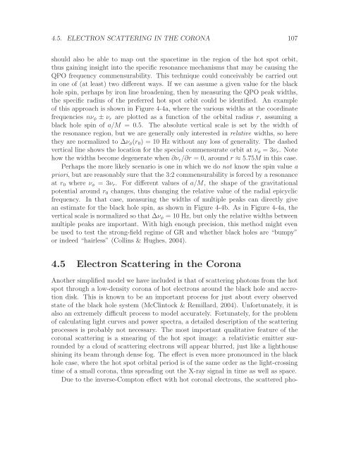
4.5. ELECTRON SCATTERING IN THE CORONA 107
should also be able to map out the spacetime in the region of the hot spot orbit,
thus gaining insight into the specific resonance mechanisms that may be causing the
QPO frequency commensurability. This technique could conceivably be carried out
in one of (at least) two different ways. If we can assume a given value for the black
hole spin, perhaps by iron line broadening, then by measuring the QPO peak widths,
the specific radius of the preferred hot spot orbit could be identified. An example
of this approach is shown in Figure 4-4a, where the various widths at the coordinate
frequencies nν φ ± ν r are plotted as a function of the orbital radius r, assuming a
black hole spin of a/M = 0.5. The absolute vertical scale is set by the width of
the resonance region, but we are generally only interested in relative widths, so here
they are normalized to ∆ν φ (r 0 ) = 10 Hz without any loss of generality. The dashed
vertical line shows the location for the special commensurate orbit at ν φ = 3ν r . Note
how the widths become degenerate when ∂ν r /∂r = 0, around r ≈ 5.75M in this case.
Perhaps the more likely scenario is one in which we do not know the spin value a
priori, but are reasonably sure that the 3:2 commensurability is forced by a resonance
at r 0 where ν φ = 3ν r . For different values of a/M, the shape of the gravitational
potential around r 0 changes, thus changing the relative value of the radial epicyclic
frequency. In that case, measuring the widths of multiple peaks can directly give
an estimate for the black hole spin, as shown in Figure 4-4b. As in Figure 4-4a, the
vertical scale is normalized so that ∆ν φ = 10 Hz, but only the relative widths between
multiple peaks are important. With high enough precision, this method might even
be used to test the strong-field regime of GR and whether black holes are “bumpy”
or indeed “hairless” (Collins & Hughes, 2004).
4.5 Electron Scattering in the Corona
Another simplified model we have included is that of scattering photons from the hot
spot through a low-density corona of hot electrons around the black hole and accretion
disk. This is known to be an important process for just about every observed
state of the black hole system (McClintock & Remillard, 2004). Unfortunately, it is
also an extremely difficult process to model accurately. Fortunately, for the problem
of calculating light curves and power spectra, a detailed description of the scattering
processes is probably not necessary. The most important qualitative feature of the
coronal scattering is a smearing of the hot spot image: a relativistic emitter surrounded
by a cloud of scattering electrons will appear blurred, just like a lighthouse
shining its beam through dense fog. The effect is even more pronounced in the black
hole case, where the hot spot orbital period is of the same order as the light-crossing
time of a small corona, thus spreading out the X-ray signal in time as well as space.
Due to the inverse-Compton effect with hot coronal electrons, the scattered pho-