Radiation Transport Around Kerr Black Holes Jeremy David ...
Radiation Transport Around Kerr Black Holes Jeremy David ...
Radiation Transport Around Kerr Black Holes Jeremy David ...

You also want an ePaper? Increase the reach of your titles
YUMPU automatically turns print PDFs into web optimized ePapers that Google loves.
146 CHAPTER 5. STEADY-STATE α-DISKS<br />
nonlinear equations<br />
f k (z n+1<br />
k+1 , zn+1 k<br />
, z n+1<br />
k−1 ) =<br />
− 1 ( z<br />
n+1<br />
k<br />
− zk<br />
n<br />
∆t n ∆t n+1/2<br />
− zn k − )<br />
zn−1 k<br />
+ pn+1 k+1/2 − pn+1 k−1/2<br />
−<br />
∆t n−1/2 Rẑˆtẑˆt<br />
∆m (r)zn+1 k<br />
= 0.(5.75)<br />
k<br />
On the right hand side, the pressure terms p n+1 are functions of the positions z n+1<br />
k+1<br />
and z n+1<br />
k−1 . The function f k is well-defined by the equations above for the interior<br />
zones (1 ≤ k ≤ N z − 1) and we use linear extrapolation to give f Nz , while planar<br />
symmetry requires z−1 n+1 = −z1 n+1 , thus defining f 0 . The solution to equation (5.75)<br />
gives the positions of the zone boundaries z n+1<br />
k<br />
, from which all the other hydrodynamic<br />
variables can be determined.<br />
Bowers & Wilson (1991) outline the standard approach to solving this set of<br />
equations using Newton-Raphson iteration and a tridiagonal solver. Denoting the<br />
first order solution to f k (t n+1 ) = 0 by the vector zk i , equation (5.75) can be written<br />
as<br />
f k (zk+1, i zk, i zk−1) i = f k (zk+1, n zk, n zk−1)<br />
n<br />
( ) n ( ) n ( ∂fk<br />
+ ∆zk+1 n + ∂fk<br />
∆zk n + ∂fk<br />
∂z n k+1<br />
∂z n k<br />
Then an approximate solution to (5.75) is<br />
∂z n k−1<br />
) n<br />
∆z n k−1 + O(∆z2 ). (5.76)<br />
z n+1<br />
k<br />
= z n k + ∆z n k. (5.77)<br />
We solve for these ∆zk n iteratively by setting f k(zk+1 i , zi k , zi k−1 ) = 0 and solving the<br />
tridiagonal system<br />
( ) n ( ) n ( ) n ∂fk<br />
− ∆zk+1 n − ∂fk<br />
∆zk n − ∂fk<br />
∆zk−1 n = f k(zk+1 n , zn k , zn k−1 ) (5.78)<br />
∂z n k+1<br />
∂z n k<br />
∂z n k−1<br />
and then re-evaluating f k (zk+1 i , zi k , zi k−1 ) until an acceptable accuracy is reached for<br />
z n+1<br />
k<br />
in equation (5.75). This typically take only about seven or eight iterations<br />
to reach machine accuracy, due to the rapid convergence of the Newton-Raphson<br />
root finding algorithm. This accuracy far exceeds the limiting first-order accuracy of<br />
the finite difference equation for energy (5.71), so we generally use only four or five<br />
iterations in the implicit scheme.<br />
As mentioned above, the technique of operator splitting is employed to model the<br />
energy transfer in the gas via radiation diffusion. Since the change in heat in a fluid<br />
element is given by dQ, the rate of energy flow due to radiation and viscous heating