Radiation Transport Around Kerr Black Holes Jeremy David ...

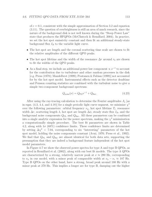
4.6. FITTING QPO DATA FROM XTE J1550–564 113
of e = 0.1, consistent with the simple approximation of Section 3.2 and equation
(3.11). The question of overbrightness is still an area of much research, since the
nature of the background disk is not well known during the “Steep Power Law”
state that produces the HFQPOs (McClintock & Remillard, 2004). In practice,
we set the hot spot emissivity constant and then fit an additional steady-state
background flux I B to the variable light curve.
• The hot spot arc length and the coronal scattering time scale are chosen to fit
the relative amplitudes of the different QPO peaks.
• The hot spot lifetime and the width of the resonance ∆r around r 0 are chosen
to fit the widths of the QPO peaks.
• As a final step, we include an additional power law component ∝ ν −1 to account
for the contribution due to turbulence and other random processes in the disk
[e.g. Press (1978); Mandelbrot (1999); Poutanen & Fabian (1999)] not accounted
for by the hot spot model. Instrumental effects such as the detector deadtime
and Poisson counting statistics are combined with the turbulent noise to give a
simple two-component background spectrum:
Q noise (ν) = Q PL ν −1 + Q flat . (4.23)
After using the ray-tracing calculation to determine the Fourier amplitudes A j [as
in eqns. (4.3, 4.4, and 4.18)] for a single periodic light curve segment, we minimize χ 2
over the following parameters: orbital frequency ν φ , hot spot lifetime T l , resonance
width ∆r, scattering length λ, hot spot arc length ∆φ, steady state flux I B , and the
background noise components Q PL and Q flat . All these parameters can be combined
into a single analytic expression for the power spectrum, making the χ 2 minimization
a computationally simple procedure. The best fit parameters are shown in Table
4.2, along with 1σ (68%) confidence limits. These confidence limits are determined
by setting ∆χ 2 < 7.04, corresponding to six “interesting” parameters of the hot
spot model, holding the noise components constant (Avni, 1976; Press et al., 1992).
We find that Q PL and Q flat are almost identical for both data sets, supporting the
presumption that they are indeed a background feature independent of the hot spot
model parameters.
In Figure 4-7 we show the observed power spectra for type A and type B QPOs, as
reported in Remillard et al. (2002), along with our best fit models. The type A QPOs
are characterized by a strong, relatively narrow peak at ν ≈ 280 Hz, corresponding
to ν φ in our model, with a minor peak of comparable width at ν φ − ν r ≈ 187 Hz.
Type B QPOs on the other hand, have a strong, broad peak around 180 Hz with a
minor peak at 270 Hz. This implies a longer arc for type B, damping out the higher