- Page 1:
Radiation Transport Around Kerr Bla
- Page 5 and 6:
5 Acknowledgments Gravity can not b
- Page 7 and 8:
Contents 1 Introduction and Outline
- Page 9 and 10:
CONTENTS 9 A Formulae for Hamiltoni
- Page 11 and 12:
List of Figures 1-1 Sample of obser
- Page 13 and 14:
List of Tables 3.1 Black hole param
- Page 15 and 16:
Chapter 1 Introduction and Outline
- Page 17 and 18:
1.2. HISTORICAL BACKGROUND 17 to th
- Page 19 and 20:
1.2. HISTORICAL BACKGROUND 19 disk
- Page 21 and 22:
1.2. HISTORICAL BACKGROUND 21 tral
- Page 23 and 24:
¼ÐÀÓÐÒÖ× 1.3. OUTLINE OF ME
- Page 25 and 26:
1.3. OUTLINE OF METHODS AND RESULTS
- Page 27 and 28:
1.3. OUTLINE OF METHODS AND RESULTS
- Page 29 and 30:
1.3. OUTLINE OF METHODS AND RESULTS
- Page 31 and 32:
1.4. ALTERNATIVE QPO MODELS 31 isot
- Page 33 and 34:
1.4. ALTERNATIVE QPO MODELS 33 jets
- Page 35 and 36:
Chapter 2 Ray-Tracing in the Kerr M
- Page 37 and 38:
2.1. EQUATIONS OF MOTION 37 Killing
- Page 39 and 40:
2.1. EQUATIONS OF MOTION 39 flat sp
- Page 41 and 42:
2.1. EQUATIONS OF MOTION 41 conveni
- Page 43 and 44:
2.1. EQUATIONS OF MOTION 43 in sepa
- Page 45 and 46:
2.2. GEODESIC RAY-TRACING 45 basis
- Page 47 and 48:
2.2. GEODESIC RAY-TRACING 47 throug
- Page 49 and 50:
2.2. GEODESIC RAY-TRACING 49 with a
- Page 51 and 52:
2.2. GEODESIC RAY-TRACING 51 since
- Page 53 and 54:
2.2. GEODESIC RAY-TRACING 53 dx µ
- Page 55 and 56:
2.2. GEODESIC RAY-TRACING 55 In the
- Page 57 and 58:
2.3. NUMERICAL METHODS 57 a long pa
- Page 59 and 60:
2.4. BROADENED EMISSION LINES FROM
- Page 61 and 62:
2.4. BROADENED EMISSION LINES FROM
- Page 63 and 64:
2.4. BROADENED EMISSION LINES FROM
- Page 65 and 66:
2.4. BROADENED EMISSION LINES FROM
- Page 67 and 68:
2.4. BROADENED EMISSION LINES FROM
- Page 69 and 70:
Chapter 3 The Geodesic Hot Spot Mod
- Page 71 and 72:
3.1. HOT SPOT EMISSION 71 Figure 3-
- Page 73 and 74:
3.1. HOT SPOT EMISSION 73 Figure 3-
- Page 75 and 76:
3.1. HOT SPOT EMISSION 75 Figure 3-
- Page 77 and 78:
3.2. NON-CIRCULAR ORBITS 77 Figure
- Page 79 and 80:
3.2. NON-CIRCULAR ORBITS 79 Figure
- Page 81 and 82:
3.2. NON-CIRCULAR ORBITS 81 paramet
- Page 83 and 84:
3.2. NON-CIRCULAR ORBITS 83 at (2/3
- Page 85 and 86:
3.2. NON-CIRCULAR ORBITS 85 form at
- Page 87 and 88:
3.3. NON-PLANAR ORBITS 87 3.3 Non-p
- Page 89 and 90:
3.3. NON-PLANAR ORBITS 89 Table 3.1
- Page 91 and 92:
3.4. SUMMARY 91 binaries in many wa
- Page 93 and 94:
Chapter 4 Features of the QPO Spect
- Page 95 and 96:
4.2. PARAMETERS FOR THE BASIC HOT S
- Page 97 and 98:
4.3. PEAK BROADENING FROM HOT SPOTS
- Page 99 and 100:
4.3. PEAK BROADENING FROM HOT SPOTS
- Page 101 and 102:
4.4. DISTRIBUTION OF COORDINATE FRE
- Page 103 and 104:
4.4. DISTRIBUTION OF COORDINATE FRE
- Page 105 and 106:
4.4. DISTRIBUTION OF COORDINATE FRE
- Page 107 and 108:
4.5. ELECTRON SCATTERING IN THE COR
- Page 109 and 110:
4.5. ELECTRON SCATTERING IN THE COR
- Page 111 and 112:
4.5. ELECTRON SCATTERING IN THE COR
- Page 113 and 114:
4.6. FITTING QPO DATA FROM XTE J155
- Page 115 and 116:
4.6. FITTING QPO DATA FROM XTE J155
- Page 117 and 118:
4.7. HIGHER ORDER STATISTICS 117 ob
- Page 119 and 120:
4.7. HIGHER ORDER STATISTICS 119 bi
- Page 121 and 122:
4.7. HIGHER ORDER STATISTICS 121 Fi
- Page 123 and 124:
4.7. HIGHER ORDER STATISTICS 123 12
- Page 125 and 126:
4.8. SUMMARY 125 els. Clearly the h
- Page 127 and 128:
Chapter 5 Steady-state α-disks The
- Page 129 and 130:
5.1. STEADY-STATE DISKS OUTSIDE THE
- Page 131 and 132:
5.1. STEADY-STATE DISKS OUTSIDE THE
- Page 133 and 134:
5.1. STEADY-STATE DISKS OUTSIDE THE
- Page 135 and 136:
5.1. STEADY-STATE DISKS OUTSIDE THE
- Page 137 and 138:
5.1. STEADY-STATE DISKS OUTSIDE THE
- Page 139 and 140:
5.2. GEODESIC PLUNGE INSIDE THE ISC
- Page 141 and 142:
5.2. GEODESIC PLUNGE INSIDE THE ISC
- Page 143 and 144:
5.3. NUMERICAL IMPLEMENTATION 143 F
- Page 145 and 146:
5.3. NUMERICAL IMPLEMENTATION 145 a
- Page 147 and 148: 5.3. NUMERICAL IMPLEMENTATION 147 (
- Page 149 and 150: 5.4. OBSERVED SPECTRUM OF THE DISK
- Page 151 and 152: 5.4. OBSERVED SPECTRUM OF THE DISK
- Page 153 and 154: 5.4. OBSERVED SPECTRUM OF THE DISK
- Page 155 and 156: 5.4. OBSERVED SPECTRUM OF THE DISK
- Page 157 and 158: Chapter 6 Electron Scattering If we
- Page 159 and 160: 6.1. PHYSICS OF SCATTERING 159 Θ
- Page 161 and 162: 6.1. PHYSICS OF SCATTERING 161 the
- Page 163 and 164: 6.1. PHYSICS OF SCATTERING 163 and
- Page 165 and 166: 6.1. PHYSICS OF SCATTERING 165 colo
- Page 167 and 168: 6.2. EFFECT ON SPECTRA 167 Let g(z)
- Page 169 and 170: 6.2. EFFECT ON SPECTRA 169 (1979);
- Page 171 and 172: 6.2. EFFECT ON SPECTRA 171 Figure 6
- Page 173 and 174: 6.3. EFFECT ON LIGHT CURVES 173 Fig
- Page 175 and 176: 6.3. EFFECT ON LIGHT CURVES 175 Fig
- Page 177 and 178: 6.3. EFFECT ON LIGHT CURVES 177 Fig
- Page 179 and 180: 6.4. IMPLICATIONS FOR QPO MODELS 17
- Page 181 and 182: Chapter 7 Conclusions and Future Wo
- Page 183 and 184: 7.1. SUMMARY OF RESULTS 183 the low
- Page 185 and 186: 7.2. CAVEATS 185 back to the coordi
- Page 187 and 188: 7.3. NEW APPLICATIONS OF CURRENT CO
- Page 189 and 190: 7.4. NEW FEATURES FOR CODE 189 grou
- Page 191 and 192: 7.5. DEVELOPMENT OF NEW MODELS 191
- Page 193 and 194: Appendix A Formulae for Hamiltonian
- Page 195 and 196: 195 The relevant spatial derivative
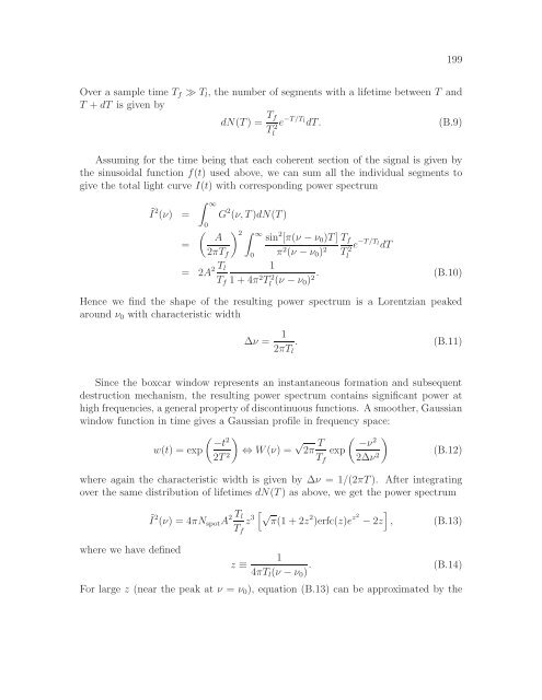
- Page 197: Appendix B Summing Periodic Functio
- Page 201 and 202: Bibliography Abramowicz, M. A., Lan
- Page 203 and 204: BIBLIOGRAPHY 203 Damour, T., & Espo
- Page 205 and 206: BIBLIOGRAPHY 205 Hawler, J. F., & G
- Page 207 and 208: BIBLIOGRAPHY 207 McClintock, J. E.,
- Page 209 and 210: BIBLIOGRAPHY 209 Psaltis, D. 2001b,
- Page 211 and 212: BIBLIOGRAPHY 211 Stern, B., et al.