PHY2014F Vibrations and Waves Part 3 - University of Cape Town

University of Cape Town
Department of Physics
PHY2014F
Vibrations and Waves
Part 3
Travelling waves
Boundary conditions
Sound
Interference and diffraction
… covering (more or less)
French Chapters 7 & 8
Andy Buffler
Department of Physics
University of Cape Town
andy.buffler@uct.ac.za
1

Problem-solving and homework
Each week you will be given a take-home
problem set to complete and hand in for marks ...
In addition to this, you need to work through the following
problems in French, in you own time, at home. You will not be
asked to hand these in for marks. Get help from you friends, the
course tutor, lecturer, ... Do not take shortcuts.
Mastering these problems is a fundamental aspect of this course.
The problems associated with Part 3 are:
7-1, 7-2, 7-3, 7-4, 7-5, 7-6, 7-7, 7-8, 7-9, 7-10, 7-11, 7-15, 7-17,
7-18, 7-19, 7-21
You might find these tougher:
2

Travelling waves
For a string clamped at both ends the displacement of the
n th normal mode is
⎛nπ
x⎞
yxt ( , ) = Asin⎜ ⎟cosω
n
t ω
n
=
⎝ L ⎠
Since L n λ nπ
vt 2π
vt
= then =
2 L λ
Then write:
And using
⎛nπ
x⎞ ⎛2π
vt⎞
ψ ( xt , ) = Asin⎜ ⎟cos⎜ ⎟
⎝ L ⎠ ⎝ λ ⎠
( ) ( )
sinα sin β = sin α + β + sin α −β
1 { }
2
A ⎛2π x 2πvt⎞ A ⎛2πx 2πvt⎞
ψ ( xt , ) = sin⎜ + ⎟+ sin⎜ − ⎟
2 ⎝ λ λ ⎠ 2 ⎝ λ λ ⎠
A ⎧ 2 π ⎫ A ⎧
sin ( x vt) sin
2 π ⎫
= ⎨ + ⎬+ ⎨ ( x−vt)
⎬
2 ⎩ λ ⎭ 2 ⎩ λ ⎭
nπ
v
L
3

Travelling waves ...2
A ⎧2π
⎫ A ⎧2π
⎫
ψ ( xt , ) = sin⎨ ( x− vt) ⎬+ sin⎨ ( x+
vt)
⎬
2 ⎩ λ ⎭ 2 ⎩ λ ⎭
A wave travelling in
the +ve x-direction
with speed v
A wave travelling in
the −ve x-direction
with speed v
The speed v is called the phase velocity and is the speed of
a crest (or any other point of specified phase) ∆x
v = ∆ t
4

Travelling waves ...3
We have shown that a standing wave
⎛nπ
x⎞ ⎛2π
vt⎞
ψ ( xt , ) = Asin⎜ ⎟cos⎜ ⎟
⎝ L ⎠ ⎝ λ ⎠
can be regarded as the superposition of two travelling waves:
A ⎧2π
ψ1( xt , ) = sin⎨
x+
vt
2 ⎩ λ
( )
⎫
⎬
⎭
and
A ⎧2π
ψ
2( xt , ) = sin⎨
x−vt
2 ⎩ λ
( )
⎫
⎬
⎭
We can think of the standing wave being made up of a travelling
wave being reflected back and forth from the two ends. The
quantity v introduced in the standing wave treatment acquires a
definite physical meaning: phase velocity
5

Formation of standing waves
…two waves having the same
amplitude and frequency,
travelling in opposite
directions, interfere with each
other.
6

Travelling waves ...4
The travelling waves we have considered are sinusoidal in shape.
Other shapes (wave pulses etc) are possible … and can be
represented as the superposition of sinusoidal waves.
Any functions f( x− vt)
or gx ( + vt)
are solutions of the
wave equation and represent travelling waves.
f
wave at time t 1 wave at time t 2
x1
x2
f( x − vt ) = f( x −vt
)
1 1 2 2
∴ x − vt = x −vt
x1−
x2
∴ v =
t − t
1 1 2 2
1 2
x
7

Travelling waves ...5
Travelling waves can be represented by sine or cosine functions:
or
⎧2π
⎫
ψ ( xt , ) = Asin⎨
( x−vt)
⎬
⎩ λ ⎭
⎧2π
⎫
ψ ( xt , ) = Acos⎨
( x−vt)
⎬
⎩ λ ⎭
⎧ ⎛ x v ⎞⎫
= Acos ⎨2π ⎜ − t ⎟⎬
⎩ ⎝ λ λ ⎠⎭
⎧ ⎛ x ⎞⎫
= Acos ⎨2π
⎜ − ft ⎟⎬
⎩ ⎝ λ ⎠⎭
wave number
2π
⎧ ⎛ x t ⎞⎫
k =
= Acos ⎨2π
⎜ − ⎟⎬
λ
⎩ ⎝ λ T ⎠⎭
= Acos{ kx − ωt}
(French: k = 1 λ ! )
8

Travelling waves ...6
Sinusoidal travelling waves:
or
or
ψ ( xt , ) = Asin{ kx− ωt+
φ}
ψ ( xt , ) = Acos kx− ωt+
φ'
{ }
ψ ( xt , ) = Asin{ kx+ ωt+
φ}
ψ ( xt , ) = Acos kx+ ωt+
φ'
{ }
waves in +ve
x-direction
waves in −ve
x-direction
λ ω
Phase velocity v phase = fλ
= 2π
f =
2π
k
9

Different types of travelling waves
“transverse”
“longitudinal”
... and water waves?
10

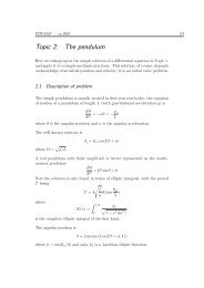
French
page 209
Wave speeds in specific media
Transverse waves on a stretched string:
Longitudinal waves in a thin rod: v =
v =
Y
ρ
T
µ
Liquids and gases: mainly longitudinal waves
Liquids:
v
B
= B: bulk modulus
ρ
Gases:
v
γ p
= =
ρ
γRT
M
γ
p
: ratio of specific heats
: pressure
11

Wave pulses
... not covered in detail.
Read French 216 - 230
12

French
page 228
Superposition of wave pulses
13

French
page 253
heavy spring
Reflection of wave pulses
light spring
very heavy spring
16

Reflection of wave pulses
heavy string light string
17

Reflection of wave pulses
Phase change of π
(i.e. inversion) on
reflection from fixed end.
No inversion on
reflection from free end.
18

Dispersion
The waves we are most familiar with (e.g. sound waves in air) are
non-dispersive … i.e. waves of different frequency travel at the
same speed.
⎧
Travelling wave on a string: 2 π ⎫
yxt ( , ) = Asin⎨
( x−vt)
⎬
⎩ λ ⎭
T
For a continuous string: v
f
n
=
µ
For a lumpy, beaded string:
= nf1
f
n
⎛ nπ
⎞
= 2f0
sin⎜ 2( N + 1)
⎟
⎝ ⎠
… high frequency waves may have a different velocity
than low frequency.
19

Dispersion …2
No dispersion of light in a vacuum.
But light is dispersed into colours by a prism:
Snell’s law:
sini
c
= n( λ)
=
sin r v( λ)
refractive index
… important for optic fibre communications …
20

French
page 213, 232 Dispersion …3
Take two sinusoidal travelling waves of slightly different frequencies:
{ ω }
{ ω }
ψ1( xt , ) = Acos
kx
1
−
1t
ψ ( xt , ) = Acos
kx−
t
2 2 2
Then ψ ( xt , ) = ψ1( xt , ) + ψ2( xt , )
where
Acos{ kx
1
ω1t} Acos{ kx
2
ω2t}
( kx− ωt) + ( kx−ω t) ( kx−ωt) −( kx−ω
t)
= − + −
⎧ ⎫ ⎧ ⎫
2Acos cos
⎩ 2 ⎭ ⎩ 2 ⎭
⎧k1+ k2 ω1+ ω2 ⎫ ⎧k1−k2 ω1−ω2
⎫
= 2Acos⎨ x− t⎬cos⎨ x−
t⎬
⎩ 2 2 ⎭ ⎩ 2 2 ⎭
1 1
= 2Acos kx −ωt cos ∆kx − ∆ωt
1 1 2 2 1 1 2 2
= ⎨ ⎬ ⎨ ⎬
k
k
{ } { }
+ k
2
ω + ω
2
2 2
1 2
1 2
= ω = 1 2
∆ k = k −k
∆ ω = ω1−ω2
21

Dispersion …4
1 1
{ } { }
ψ ( xt , ) = 2Acos kx−ωt cos ∆kx− ∆ωt
2 2
Average
travelling wave
Envelope
{ − ωt}
cos{ 1 ∆kx − 1 ∆ωt}
cos kx
ω
v phase = ∆ω
2
k
Group velocity = v group =
∆k
2
2 2
=
∆ω
∆k
22

Dispersion …5
Phase velocity:
Group velocity:
v phase =
v group =
ω
k
∆ ω =
∆k
dω
dk
… the wave packet moves at v g … so does transport of energy
When analyzing an arbitrary pulse into pure sinusoids …
… if these sinusoids have different characteristic speeds, then
the shape of the disturbance must change over time …
… a pulse that is highly localized at t = 0 will become more
and more spread out as it moves along.
23

Dispersion …6
Consider surface waves on liquids …
For long wavelength waves (λ ~ m) on deep water (gravity waves):
ω =
gk
then
v
g
ω
vφ
= =
k
dω
1
= =
dk 2
g
k
g
k
∴ v =
φ
1
v
2 g
For short wavelength waves (λ ~ mm) on deep water
(capillary waves or ripples):
ω Sk
S vφ
= =
ω = k
3
then k ρ
ρ
∴ v
3
φ
= v
dω
3 Sk
vg
= =
dk 2 ρ
S = surface tension
2 g
24

Phase and group velocities of a wave and a pulse
with
= φ
2v
g
v
25

French
page 237
The energy in a mechanical wave
Consider a small segment
of a string carrying a wave:
ds
T
dy
Mass of segment = µ dx
T
dx
y
If u = ∂
y
x
x+
dx x
∂ t
dK 1 ⎛ y
2
µ ∂ ⎞
then kinetic energy per unit length = = ⎜ ⎟
dx 2 ⎝ ∂t
⎠
Potential energy = Tds ( − dx)
2 2
2 2 ∂y
⎛ 1 ∂y
⎞
where
⎛ ⎞ ⎛ ⎞
ds = dx + dy = dx 1+ ⎜ ⎟ = dx
1 + ⎜ ⎟ + ...
⎝∂x⎠ ⎜ 2 ⎝∂x⎠
⎟
⎝
⎠
2
dU 1 ⎛∂y
⎞
Then potential energy per unit length = = T ⎜ ⎟ 26
dx 2 ⎝∂x
⎠

The energy in a mechanical wave …2
⎧ ⎛
For a travelling wave on a string: yxt ( , ) = Asin⎨2π
f⎜t−
⎩ ⎝
∂y
⎧ ⎛ x ⎞⎫
Then uy
( x, t) = = 2π
fAcos⎨2π
f ⎜t−
⎟⎬
∂t
⎩ ⎝ v⎠⎭
cos ⎧
2 ⎛ x ⎞⎫
= u0 ⎨ π f ⎜t−
⎟⎬
⎩ ⎝ v ⎠⎭
∂y ⎧2π
fx⎫ ⎧2π
x⎫
At t = 0: uy
( x) = = u0cos⎨ ⎬=
u0cos⎨ ⎬
∂t
⎩ v ⎭ ⎩ λ ⎭
then
2
dK 1 ⎛∂
y ⎞ 1 2 2⎧2π
µ µ u0
cos
x ⎫
= ⎜ ⎟ = ⎨ ⎬
dx 2 ⎝ ∂t
⎠ 2 ⎩ λ ⎭
x
v
⎞⎫
⎟⎬
⎠⎭
and
λ
1 ⎧2π
x ⎫ 1
K = ∫ µ u cos dx=
λµ u
2 ⎩ λ ⎭ 4
0
2 2 2
0 ⎨ ⎬
0
in one wavelength
27

The energy in a mechanical wave …3
Similarly for potential energy:
At t = 0:
∂y 2π
A ⎧2π
x⎫
=− cos ⎨ ⎬
∂x
λ ⎩ λ ⎭
then
and
2 2
2π
2 ⎧2
cos
2
dU A T π x ⎫
= ⎨ ⎬
dx λ ⎩ λ ⎭
λ
2 2 2 2
2π A T 2 ⎧2πx⎫
2π
A T λ
U = ∫ cos dx
2 ⎨ ⎬ =
in one wavelength
2
λ λ λ 2
0
⎩ ⎭
2 2 2 1 2
∴ U = π A µ f λ = λµ u u0 = 2π
fA
0
4
Over one wavelength, total energy:
1
E = K + U = λµ u
2
2
0
28

French
page 241
θ
F
Transport of energy
y 0
by a wave
⎧ ⎛ x ⎞⎫
yxt ( , ) = Asin⎨2π
f⎜t−
⎟⎬
⎩ ⎝ v ⎠⎭
A long string has one end at x = 0 and is driven at this point by a
driving force F equal in magnitude to the tension T and applied
in a direction tangent to the string.
At x = 0 : y(0, t) = Asin 2π
ft
⎛∂y⎞ ⎛ 2π
fA ⎞
and Fy
=−Tsinθ
≈− T⎜ ⎟ =−T⎜−
cos 2π
ft ⎟
⎝∂x⎠x=
0 ⎝ v ⎠
Then work done:
2π
fAT
W = ∫Fydy0
= ∫ cos 2 π ft d Asin 2π
ft
v
2
( 2π
fA)
T
(
2
= ∫ cos 2π
ft)
dt 29
v
( ) ( )
x

Transport of energy by a wave …2
For one complete cycle: from t = 0 to t = 1/f :
2 1 f
2
uT
0
uT
0
1 2
cycle
= ∫ (1+ cos4 π ) = = λµ
0
2v
2vf
2
0
W ft dt u
Then mean power input P =
W
uT 1
2v
2
2
1 0
2
cycle
= = µ
0
f
u v
…thusP = energy per unit length × velocity
… energy flows along medium at velocity v …
…and at v g if the medium is dispersive
30

Doppler effect
... frequency changes of traveling waves due to motion of source
and/or detector ...
S: source of waves (sound)
λ
D: detector
S D
v S : speed of source
v D
: speed of detector
v
v : speed of travelling wave = f λ
When both vS
and vD
are
zero,then the number of
wavelengths
vt
passing D in time t is
λ
S
v D
D
31

Doppler effect ...2
For the case of stationary S and moving D:
For moving D we must add (or
subtract) vtλ
D wavelengths.
S
v D
v
D
vt λ ± vDt
Observed frequency: f ' =
t
v±
v
= D
λ
Source frequency: f = v λ
λ
∴ f ' =
f
v
± v
v
D
32

Doppler effect ...3
For the case of moving S and stationary D:
In time period T, S moves a
distance vT
S
.
Wavelength at D is therefore
shortened (or lengthened) by vT.
Observed wavelength: λ ' = λ ∓
v v vS
v vS
∴ = ∓ = ∓
f ' f f f
v
∴ f ' = f v ∓ v
S
S
vS
For both source and detector moving:
v±
vD
f ' = f v ∓ v
S
f
S
v S
D
D
33

Doppler effect ...4
At supersonic speeds v > v , this relationship no longer applies:
All wavefronts are buched along a
V-shaped envelope in 3D ... called a
Mach cone ... a shock wave exists
alongs the surface of this cone since the
bunching of the wavefronts causes an
abrupt rise and fall of air pressure as the
surface passes any point ... causes a
“sonic boom”
S
vS
=
v
vS
= v
vS
>
v
vt
θ
vt
sinθ = =
vt
S
v
v
S
vt
S
“Mach number”
34

Doppler effect ...5
supersonic
aircraft
travelling
bullet
bow wave
of a boat
... get a “sonic boom” whenever
the speed of the source of the
waves is greater than the speed of
waves in that medium.
Cherenkov
radiation
35

Doppler effect ...6
36

Physical optics
Electromagnetic radiation can be modelled as a wave or a beam of
particles ... all observed phenomena can be described by either model,
although the treatment my be easier with one, or the other.
EM radiation propagates in vacuo, and may be thought of as E and
B fields in phase with each other, and propagating at right angles
to each other and to the direction of propagation.
Velocity of EM radiation in vacuum = constant, c
In a medium of refractive index n, v=
c n
EM wave from a point source:
E is in phase around each circle ...
vacuum
c
... get a coherent plane
wave at a large distance
from point source
37

Interference
If we use two in-phase sources to
generate waves on the surface of a
liquid it is easy to observe
interference effects. At certain
points the waves are in phase and
add constructively, and at other
points they are out of phase,
interfere destructively, giving zero
amplitude.
... this is not an everyday observation with light sources ... the
wavelength of light is small (400-800 nm) ... ordinary light
sources are enormously larger than this ... and are not
monochromatic.
38

Try this ...?
filter
double
slit
Interference ...2
screen
... no interference
fringes observed ...
light from different
portions of source is
incoherent ... no fixed
phase relationship
Thomas Young performed a classic interference experiment in 1801:
... interference fringes
observed on screen ...
filter
pinhole
double
slit
screen
39

Interference ...3
... but why do we see fringes at all ...
doesn’t light travel in straight lines?
Huyghens showed that one could
regard each point on a wavefront as
being a source of “secondary wavelets”
... the envelope of these secondary
wavelets form a subsequent wavefront
...
wavefronts
40

Huyghens’ Principle
screen
plane
wave
travelling
in this
direction
Aperture large compared with
a wavelength
... some spreading of wave
Aperture similar size
to a wavelength ...
large angular spread
from small aperture
41

Young’s double slit experiment
back to Young’s
experiment ...
... the two slits in
the second screen
act as coherent
sources
42

Young’s double slit experiment ...2
d
θ
y
D
screen
Path difference = d sinθ
Maxima on screen when
Minima on screen when
dsinθ
= mλ
1
( m )
dsinθ
= +
y = Dsinθ
for small θ
mλ
∴ y = D for maxima
d
2
λ
m = 0, ±1, ±2, ...
43

Young’s double slit experiment ...3
... a more detailed treatment
d
r
r 2
θ
P
r 1
Suppose a plane wave illuminates the slits ... the waves from
the two slits are in phase at the slits.
Since the distances r 1 and r 2 differ, the waves will have a phase
difference at P.
E1 = E0cos( kr1−ω
t)
Electric fields of the two waves:
E = E cos( kr −ωt)
2 0 2
... both waves have the same amplitude at P ... not quite right
since r 1 and r 2 are different distances ... but ok.
44

Young’s double slit experiment ...4
Total field: E = E1+ E2 = E0cos( kr1− ωt) + E0cos( kr2
−ωt)
( + ) ( − )
⎧k r1 r2 ⎫ ⎧k r1 r2
⎫
= 2E0
cos⎨ −ωt⎬cos⎨ ⎬
⎩ 2 ⎭ ⎩ 2 ⎭
⎧k
⎫
= 2E0
cos{ kr−ωt}
cos⎨ dsinθ
⎬
⎩2
⎭
⎧π
d ⎫
= 2E0
cos{ kr−ωt}
cos⎨ sinθ
⎬
⎩ λ ⎭
2
2
We now take (time average of )
I
=
E
E
Thus for one slit only:
similarly:
E
2
2 2 0
1
=
0cos (
1− ω ) =
I E kr t
I =
2
E
2
0
2
2
45

Young’s double slit experiment ...5
2
Write
1
I = I = I = E
0 1 2 2 0
2 2 2⎧π
d ⎫
= 4
0
cos − cos ⎨ sinθ
⎬
⎩ λ ⎭
2⎧π
d ⎫
2φ
∴ I = 4I0cos ⎨ sinθ
⎬=
4I0cos ⎩ λ ⎭ 2
2 π d
So I will have maxima when cos ⎧ ⎨ sinθ
⎫ ⎬ = 1
⎩ λ ⎭
π d
or when sinθ
= mπ
m = 0, ±1, ±2, ...
λ
For both slits: I E { kr ωt}
or dsinθ
= mλ
This approach gives us additional information ...
46

Young’s double slit experiment ...6
Double slit interference pattern
I
two sources
(coherent)
two sources
(incoherent)
single source
⎧π
d ⎫
= I ⎨ θ ⎬
⎩ λ ⎭
2
( θ ) 4
0
cos sin
I
4I 0
2I 0
I 0
m =
π d
sinθ
=
λ
−3 −2 −1 0 1 2 3
−3π −2π −π 0 π 2π 3π
47

Young’s double slit experiment ...7
... can also use phasors ...
Ψ =
Ae
1 0
Ψ jkr ( 2−ωt)
( −ωt)
jkr
1
Ψ =
2 0
δ =
Ae
Ae
0
( − ωt+
δ )
jkr
1
Ψ
Ψ 2
Ψ 1
Ψ 1
Ψ
Ψ 2
Ψ( δ )
2A 0
Ψ
Ψ 1
Ψ 2
0 π 2π
δ
Ψ = 0
Ψ 2
Ψ 1
48

Interference patterns from thin films
“Black” (i.e. destructive intereference)
from very thin film indicates that there is a
phase change of π at one of the reflections.
t
λ
For wedges having small angle α , bright fringes correspond to an
increase of λ 2 in thickness t :
For nearly normal incidence,
x
t λ path difference = 2t
dark
Minima occur when the
π out of phase
t = λ 4 path difference = nλ
bright
2π out of phase
dark
3π out of phase
t
= λ 2
For minima, 2t = nλ
or 2x
n
α = nλ
Distance between fringes:
49
x − n 1
x =
+ n
λ 2α

To obtain fringes on a visible scale a very
small angle is necessary ... such fringes may
be seen on viewing the light reflected from a
soap film held vertically as it “drains” ...
For other interference effects, look up for yourself:
Lloyd’s mirror
Fresnel bi-prism
S 1
S
fringes
S
fringes
S 2 S 1
Michelson
interferometer
fringes
Newton’s rings
fringes
50

Fresnel diffraction
Around 1818 Augustin Fresnel applied Huyghen’s
priciple to the problem of diffraction of light by
apertures and obstacles ... took into account the
realtive phases of the secondary wavelets
consequent upon their having to travel diferent
distances to the point of observation ... analytical
treatment is complicated
... look at the results of a few special cases ...
Shadow of a straight edge
(cast by a point source S)
... no sharp edge to the shadow
... illumination diminishes
smoothly into the shadow
... with fringes outside the
shadow.
S
51

Shadow of a narrow slit: centre of
pattern at P may either be a relative
maximum or minimum, depending on
ratio of slit width to wavelength.
Shadow of a narrow parallel-sided
obstacle: centre always a relative
maximum ... but very faint unless
obstacle is very narrow.
S
S
Shadow of a circular obstacle: wavelets from all round
circumference all reinforce at centre of shadow.
S
“Poisson” bright spot
(found by Arago)
52

Fraunhofer diffraction
... special (limiting) cases of Fresnel
diffraction ... when both the distances
to source and screen both tend to
infinity ... treatment is easier since the
paths of all the wavelets to any point
of interest are parallel.
It is practical sometimes to use a lens ... what would be seen at
infinity is then found in its focal plane.
or
S
53

Fraunhofer diffraction
by a single slit
Let slit width be a
... picture below very
much distorted in scale...
incident
wave
y
a
2
dy
θ
r
r 0
P
−a
2
ysinθ
To find the intensity of the wave at P we “add” the contributions
at P of waves originating from all points of the aperture.
a 2 a 2
jkr−ω jkr− t−jkysinθ
Ψ ( P)
= ∫
=
( t) ( ω )
0
Ae dy A e dy
−a
2 −a
2
∫
a 2
jkr t jky
( −ω
)
= ∫
0
− sinθ
Ae e dy
−a
2
54

Fraunhofer diffraction by a single slit ...2
Ψ ( P)
=
a 2
jkr ( −ωt)
∫
0
jky
−a
2
0
− sinθ
A e e dy
( −ω
)
⎡ 1
⎣−
jk sinθ
jkr t jky
0
− sinθ
= Ae
0 ⎢ e ⎥
=
∴Ψ ( P)
=
a
a
jk sinθ
− jk sinθ
2 2
jkr ( 0−ωt)
e − e
Ae
0
jk sinθ
⎡
⎢use sinφ
=
⎣
Then
Ae
I =Ψ
2 ( P)
⎤
⎦
a
2
−a
1
( −ω
) sin( 2
sinθ
)
jkr t ka
0
a
0 1
2
I( θ )
e
jφ
I
− e
2 j
− jφ
⎤
⎥
⎦
⎛sinα
⎞
⎝ α ⎠
∴ =
0 ⎜ ⎟
kasinθ
2
2
where
⎛sinα
⎞
⎜ ⎟
⎝ α ⎠
1
α =
2
kasinθ
55
α

I( θ )
Fraunhofer diffraction by a single slit ...3
I
⎛sinα
⎞
⎝ α ⎠
∴ =
0 ⎜ ⎟
2
1
where α =
2
kasinθ
I 0
I( θ )
α = −3π −2π −π 0 π 2π 3π
λ λ λ
sinθ = −3 λ λ λ
−2 −
2 3 a a a a a a
Minima at
or
α =
mπ
1
2
kasinθ
= mπ
where
or
m = ±1, ±2, ...
m 2π
λ
sinθ = = m
a k a
56

Fraunhofer diffraction by a single slit ...4
Using phasors ... consider a single slit as N sources, each of
amplitude A 0 ... in the example below, N = 10.
The path difference between any two adjacent sources is d sinθ
where d = a N and the phase difference is δ = dk sinθ
.
At the central maximum
point at θ = 0 , the waves
from the N sources add in
phase, giving the resultant
amplitude A = NA .
max 0
At the first minimum, the N phasors form a
closed polygon ... the phase difference
between adjacent sources is then δ = 2π
N
When N is large, the waves from the first
and last sources are approximately in phase
A 0
A
=
NA
max 0
δ =
57
2π
N

Fraunhofer diffraction by a single slit ...5
At a general point
... where the waves from
two adjacent sources differ
in phase by δ ...
The phase difference
between the first and last
wave is φ .
r
r
φ 2
φ 2
A
φ
As N increases, the phasor diagram approximates the arc of a circle
... the resultant amplitude A is the length of the chord of this arc.
( )
The length of the arc is A ( = NA )
1
From the figure: sin φ 2 = A 2r
or A = 2r sin 2
φ
A max
max 0
Therefore φ = or
r
r
=
Amax
φ
58

Fraunhofer diffraction by a single slit ...6
1
A
1 max
sin
1
2
φ
Combining ... A= 2rsin φ = 2 sin φ = Amax
φ
φ
Then
I
I
⎛ φ ⎞
= = ⎜ ⎟
⎝ φ ⎠
2 1
A sin 2
2 1
0
A max 2
2 2 1
2
2
or I
⎛
1
sin 2
φ ⎞
= I0 ⎜ 1 ⎟
⎝ 2
φ ⎠
...where φ is the phase difference between the
first and last waves = 2π λ asinθ = kasinθ
( )
2
The second maximum occurs when the N
1
phasors complete circles:
1 2
A
... and the resultant amplitude is the diameter of the circle ...
2
2
C
3
Amax 2Amax
2 4Amax
The diameter A = = = then A =
2
π π 3 π
9π
4 1
and I = I0 = I
2 0
9π
22.2
59

Interference and diffraction from a double slit
When there are two or more slits, the intensity pattern on a
screen far away is a combination of the single slit diffraction
pattern and the multiple slit interference pattern.
2
⎛sinα
⎞
= I0
⎜ ⎟
I( θ ) 4 cos
⎝ α ⎠
2
β
π a
α = sinθ
λ
π d
β = sinθ
λ
60

Interference and diffraction from a double slit ...2
intensity pattern
for two slits
if a → 0 :
intensity pattern
for one slit of
width a :
intensity pattern
for two slits
each of width a :
sinθ =
−2 a
λ
λ
−
a
λ
−3 d
−2 d
λ
λ
−
d
0
λ
2 d
λ
d
λ
a
λ
3 d
61
2 a
λ

Interference patterns from multiple slits (diffraction gratings)
d
... many slits, with inter-slit spacing d,
illuminated by a plane wave ...
As with the double slit, each slit acts as a
source of waves.
Consider each pair of slits as a Young’s double slit.
Slits are coherent, in phase sources for light at an
angle θ to the n th n
bright fringe.
For constructive interference
d
sinθ
n
= nλ
n = 0, ±1, ±2, ...
If m is the number of slits, then amplitude at θn
is A = ma
where a is the amplitude form a single slit
2 2 2
Then I ∼ A ∼m
a (...many slits give intense fringes)
62

Interference patterns from multiple slits ...2
d sinθ
θ
r 1
r 2
r 3
r 4
to P
r2 = r1+
dsinθ
r3 = r2 + 2dsinθ
r4 = r1+
3dsinθ
etc.
Total field at P:
E = E1+ E2 + E3 + ...
= E cos( kr − ωt) + E cos( kr − ωt) + E cos( kr − ωt) + ...
0 1 0 2 0 3
Use complex numbers:
( −ω ) ( −ω ) jkr ( −ωt)
E = E e + E e + E e +
jkr1 t jkr2
t
3
0 0 0
...
63

Interference patterns from multiple slits ...3
( −ω ) ( −ω ) jkr ( −ωt)
E = E e + E e + E e +
jkr1 t jkr2
t
3
0 0 0
...
( − ω ) ( − ω + sin θ ) ( − ω + 2 sin θ )
= Ee + Ee + Ee
+
j kr1 t j kr1 t kd j kr1
t kd
0 0 0
...
( )
{ }
1−ω sinθ 2 sin θ ( −1) sinθ
jkr t jkd jkd N jkd
= Ee
0
1 + e + e + ... + e
... for N slits
∴ E =
=
E e
geometric progression
(
jkd sinθ
1−
e )
( −ωt) jkr1
0 jkd sinθ
Ee
1−
e
N
N N N
2 2 2
jkd sinθ (
− jkd sinθ jkd sinθ
e e − e )
( −ωt) jkd θ
(
− jkd θ jkd θ
e e − e )
jkr1
0 sin sin sin
1 1 1
2 2 2
jφ
− jφ
e − e
and using sinφ
=
...
2 j
64

Interference patterns from multiple slits ...4
∴ E = E e E e
1
N −1
( ) ( )
1−ω
jkd sinθ
sin
2
2
sinθ
sin( kd sinθ
)
jkr t Nkd
0 0 1
2
=
Ee
0
N −
{ ( 1+ 1 sin
2 ) − }
sin
sin β
jkr jkd θ ωt Nβ
Write
E
=
E e
0
{ −ω
}
sin β
sin β
jkr t N
where
π d
2
sin sin
λ
1
β = kd θ = θ
Then, as before,
I( θ )
I
⎛sin
Nβ
⎞
⎝ sin β ⎠
=
0 ⎜ ⎟
2
65

Interference patterns from multiple slits ...5
I( θ )
I
⎛sin
Nβ
⎞
⎝ sin β ⎠
=
0 ⎜ ⎟
2
β =
π d
sinθ
λ
I
N = 2
N = 3
N = 4
π d
sinθ
= −3π −2π −π 0 π 2π 3π
λ
66

Interference patterns from multiple slits ...6
Phasors for a 10 slit grating (N = 10) ...
δ =
0,2π
δ = 2π
N = 36°
Ψ( δ )
10A 0
δ = 4π
N = 72°
δ = 3π
N = 54°
δ = 5π
N = 90°
0 π 2π
δ
δ = 6π
N = 108° δ = 7π
N = 126°
67

Circular apertures
Different shaped apertures will give
different diffraction patterns.
A commonly encountered aperture in
optics is the circular aperture.
... diffraction pattern described by
a Bessel function, with the first
minimum at
λ
sinθ = 1.22 d
... where d is the diameter
To resolve two objects,
−1
λ
where θR
= sin 1.22
d
Rayleigh criterion
θ > θ R
θ
θ < θ
> θR
θ = θR
R
68

Interference and diffraction with water waves
See French 280 - 294
69