Numerical simulation of the heat transfer in amorphous ... - Physics
Numerical simulation of the heat transfer in amorphous ... - Physics
Numerical simulation of the heat transfer in amorphous ... - Physics

You also want an ePaper? Increase the reach of your titles
YUMPU automatically turns print PDFs into web optimized ePapers that Google loves.
4396 Rev. Sci. Instrum., Vol. 74, No. 10, October 2003 Revaz et al.<br />
mal conduction layer <strong>in</strong> <strong>the</strong> sample area is to underestimate<br />
<strong>the</strong> real <strong>the</strong>rmal conductivity <strong>of</strong> <strong>the</strong> membrane or sample by<br />
<strong>the</strong> fractional change shown <strong>in</strong> Fig. 3; for k 2D,Cu /k 2D,m<br />
100, this is 1.5% <strong>the</strong> % decrease <strong>in</strong> P/T for T2 at<br />
f<strong>in</strong>ite k 2D,Cu /k 2D,m compared to <strong>the</strong> extremely high<br />
k 2D,Cu /k 2D,m limit which is with<strong>in</strong> <strong>the</strong> uncerta<strong>in</strong>ty <strong>in</strong> film<br />
thickness for most cases. It is also possible to use <strong>the</strong> simulated<br />
P/T values shown <strong>in</strong> Fig. 3 to make a correction by<br />
extract<strong>in</strong>g <strong>the</strong> geometric factor connect<strong>in</strong>g a given P/T for<br />
T1 or T2 with k 2D,m , at least <strong>in</strong> <strong>the</strong> limit where <strong>the</strong> sample<br />
area is nearly iso<strong>the</strong>rmal large but not <strong>in</strong>f<strong>in</strong>ite (k 2D,s<br />
k 2D,m )/k 2D,m ], s<strong>in</strong>ce Fig. 3 is at constant k 2D,m . For example,<br />
at a ratio <strong>of</strong> 100, a common lower limit for <strong>the</strong> devices<br />
reached through use <strong>of</strong> a Cu conduction layer, <strong>the</strong> contour<br />
l<strong>in</strong>es <strong>of</strong> Fig. 2 and <strong>the</strong> <strong>simulation</strong> data <strong>in</strong> Fig. 3 show<br />
that <strong>the</strong> geometrical factor is reduced from 10.33 to 10.0 for<br />
T2 <strong>the</strong> same 1.5% correction.<br />
B. Time dependence: PÄ0<br />
In this section, we turn to <strong>the</strong> analysis <strong>of</strong> <strong>the</strong> relaxation<br />
T(t). Experimentally, <strong>the</strong> relaxation is measured by<br />
switch<strong>in</strong>g <strong>of</strong>f at time t0) <strong>the</strong> current flow<strong>in</strong>g <strong>in</strong> <strong>the</strong> <strong>heat</strong>er<br />
and record<strong>in</strong>g <strong>the</strong> relaxation <strong>of</strong> <strong>the</strong> <strong>of</strong>f-null voltage across<br />
<strong>the</strong>rmometers T1 and T2, us<strong>in</strong>g an ac bridge described <strong>in</strong><br />
Ref. 4. In <strong>the</strong> high ratio limit (k 2D,s k 2D,m )/k 2D,m 1 produced<br />
by a parallel <strong>the</strong>rmal conduction layer such as <strong>the</strong><br />
1800 Å <strong>of</strong> Cu used here <strong>in</strong> measurement 3, we have previously<br />
shown experimentally that a s<strong>in</strong>gle time constant is<br />
seen, out to 7 ext . 4<br />
We start by compar<strong>in</strong>g <strong>simulation</strong> and experiment <strong>of</strong> <strong>the</strong><br />
time dependence for <strong>the</strong> empty calorimeter <strong>in</strong> order to extract<br />
<strong>the</strong> specific <strong>heat</strong> <strong>of</strong> <strong>the</strong> a-Si–N membrane at 20.3 K, <strong>the</strong><br />
temperature chosen for absolute calibration purposes. We<br />
<strong>the</strong>n turn to <strong>simulation</strong>s <strong>of</strong> <strong>the</strong> relaxation response <strong>of</strong> <strong>the</strong><br />
membrane with a sample <strong>of</strong> various <strong>the</strong>rmal conductivity and<br />
specific <strong>heat</strong>. We show that even for a relatively low ratio <strong>of</strong><br />
sample to membrane <strong>the</strong>rmal conductivity, fits to a s<strong>in</strong>gle<br />
time constant can be used to extract <strong>the</strong> sample <strong>heat</strong> capacity,<br />
and we derive <strong>the</strong> systematic errors <strong>in</strong>troduced by this<br />
method as a function <strong>of</strong> this ratio. We also derive <strong>the</strong> contributions<br />
to <strong>the</strong> total <strong>heat</strong> capacity <strong>of</strong> <strong>the</strong> membrane border and<br />
<strong>the</strong> Pt leads. We <strong>the</strong>n study <strong>the</strong> differential method directly,<br />
simulat<strong>in</strong>g a an <strong>in</strong>itial sample layer e.g., <strong>of</strong> Cu, followed<br />
by a second identical layer, as <strong>in</strong> a calibration measurement,<br />
and b with <strong>the</strong> second layer be<strong>in</strong>g a more normal sample<br />
with high <strong>heat</strong> capacity but relatively low <strong>the</strong>rmal conductivity.<br />
The systematic error <strong>in</strong> this differential method is shown<br />
to be less than <strong>in</strong> <strong>the</strong> s<strong>in</strong>gle layers, and is derived as a function<br />
<strong>of</strong> <strong>the</strong> ratio <strong>of</strong> <strong>in</strong>ternal to external <strong>the</strong>rmal conductivity<br />
and sample to membrane specific <strong>heat</strong>. This systematic error<br />
is shown to be less than 2% under standard operat<strong>in</strong>g conditions<br />
<strong>of</strong> a Cu conduction layer with thickness equal to that <strong>of</strong><br />
<strong>the</strong> membrane. F<strong>in</strong>ally, a method for an iterative correction<br />
for this systematic error is discussed.<br />
1. Empty calorimeter: Membrane <strong>heat</strong> capacity<br />
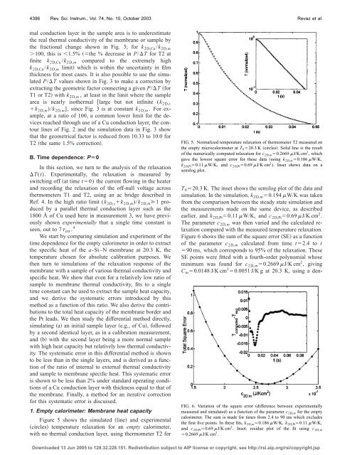
Figure 5 shows <strong>the</strong> simulated l<strong>in</strong>e and experimental<br />
circles temperature relaxation for an empty calorimeter,<br />
with no <strong>the</strong>rmal conduction layer, us<strong>in</strong>g <strong>the</strong>rmometer T2 for<br />
FIG. 5. Normalized temperature relaxation <strong>of</strong> <strong>the</strong>rmometer T2 measured on<br />
<strong>the</strong> empty microcalorimeter at T 0 20.3 K circles. Solid l<strong>in</strong>e is <strong>the</strong> result<br />
<strong>of</strong> <strong>the</strong> numerically computed relaxation for c 2D,m 0.2669 J/K cm 2 , which<br />
gave <strong>the</strong> lowest square error for <strong>the</strong>se data us<strong>in</strong>g k 2D,m 0.186 W/K,<br />
k 2D,Pt 0.11 W/K, and c 2D,Pt 0.69 J/K cm 2 ). Inset shows data on a<br />
semilog plot.<br />
T 0 20.3 K. The <strong>in</strong>set shows <strong>the</strong> semilog plot <strong>of</strong> <strong>the</strong> data and<br />
<strong>simulation</strong>. In <strong>the</strong> <strong>simulation</strong>, k 2D,m 0.194 W/K was taken<br />
from <strong>the</strong> comparison between <strong>the</strong> steady state <strong>simulation</strong> and<br />
<strong>the</strong> measurements made on <strong>the</strong> same device, as described<br />
earlier, and k 2D,Pt 0.11 W/K, and c 2D,Pt 0.69 J/K cm 2 .<br />
The parameter c 2D,m was <strong>the</strong>n varied and <strong>the</strong> calculated relaxation<br />
compared with <strong>the</strong> measured temperature relaxation.<br />
Figure 6 shows <strong>the</strong> sum <strong>of</strong> <strong>the</strong> square error SE as a function<br />
<strong>of</strong> <strong>the</strong> parameter c 2D,m calculated from time t2.4 to t<br />
90 ms, which corresponds to 95% <strong>of</strong> <strong>the</strong> relaxation. These<br />
SE po<strong>in</strong>ts were fitted with a fourth-order polynomial whose<br />
m<strong>in</strong>imum was found for c 2D,m 0.2669 J/K cm 2 , giv<strong>in</strong>g<br />
C m 0.0148 J/K cm 3 0.0051 J/K g at 20.3 K, us<strong>in</strong>g a den-<br />
FIG. 6. Variation <strong>of</strong> <strong>the</strong> square error difference between experimentally<br />
measured and simulated as a function <strong>of</strong> <strong>the</strong> parameter c 2D,m for <strong>the</strong> empty<br />
calorimeter. The sum is made for times from 2.4 to 90 ms which excludes<br />
<strong>the</strong> first five po<strong>in</strong>ts. In <strong>the</strong>se fits, k 2D,m 0.186 W/K, k 2D,Pt 0.11 W/K,<br />
and c 2D,Pt 0.69 J/K cm 2 . Inset: residue plot <strong>of</strong> <strong>the</strong> fit us<strong>in</strong>g c 2D,m<br />
0.2669 J/K cm 2 .<br />
Downloaded 13 Jun 2005 to 128.32.228.151. Redistribution subject to AIP license or copyright, see http://rsi.aip.org/rsi/copyright.jsp