PhD Thesis - Universität Augsburg
PhD Thesis - Universität Augsburg
PhD Thesis - Universität Augsburg

Create successful ePaper yourself
Turn your PDF publications into a flip-book with our unique Google optimized e-Paper software.
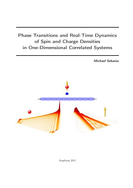
Phase Transitions and Real-Time Dynamics<br />
of Spin and Charge Densities<br />
in One-Dimensional Correlated Systems<br />
Michael Sekania<br />
<strong>Augsburg</strong> 2011
Phase Transitions and Real-Time Dynamics<br />
of Spin and Charge Densities<br />
in One-Dimensional Correlated Systems<br />
Dissertation<br />
zur Erlangung des Grades eines<br />
Doktors der Naturwissenschaften<br />
(Dr. rer. nat.)<br />
eingereicht an<br />
der Mathematisch-Naturwissenschaftlichen Fakultät<br />
der <strong>Universität</strong> <strong>Augsburg</strong><br />
von M.Sc.<br />
Michael Sekania<br />
aus Tbilisi (Tiflis), Georgien<br />
<strong>Augsburg</strong> 2011
Erstgutachter:<br />
Zweitgutachter:<br />
Prof. Dr. Arno P. Kampf<br />
Prof. Dr. Thilo Kopp<br />
Tag der Einreichung: 17. Januar 2011<br />
Tag der mündlichen Prüfung: 03. Juni 2011
Contents<br />
i<br />
CONTENTS<br />
Introduction . . . . . . . . . . . . . . . . . . . . . . . . . . . . . . . . . . . . . . . 1<br />
1. Models . . . . . . . . . . . . . . . . . . . . . . . . . . . . . . . . . . . . . . . . 7<br />
1.1 Model Hamiltonian for electrons in solids . . . . . . . . . . . . . . . . . . . 7<br />
1.2 Hubbard model . . . . . . . . . . . . . . . . . . . . . . . . . . . . . . . . . 12<br />
1.3 t-J and Heisenberg models . . . . . . . . . . . . . . . . . . . . . . . . . . . 18<br />
1.4 Extended Hubbard models . . . . . . . . . . . . . . . . . . . . . . . . . . . 20<br />
1.4.1 Next-nearest neighbor interaction . . . . . . . . . . . . . . . . . . . 21<br />
1.4.2 Peierls distortion . . . . . . . . . . . . . . . . . . . . . . . . . . . . 21<br />
1.4.3 Ionic potential . . . . . . . . . . . . . . . . . . . . . . . . . . . . . . 21<br />
2. Density-Matrix Renormalization Group . . . . . . . . . . . . . . . . . . . . . 23<br />
2.1 Introduction . . . . . . . . . . . . . . . . . . . . . . . . . . . . . . . . . . . 23<br />
2.2 Matrix-Product State . . . . . . . . . . . . . . . . . . . . . . . . . . . . . . 24<br />
2.2.1 MPS, Blocks, and a Superblock . . . . . . . . . . . . . . . . . . . . 28<br />
2.2.2 Operators in block effective basis . . . . . . . . . . . . . . . . . . . 30<br />
2.3 Density-Matrix Projection . . . . . . . . . . . . . . . . . . . . . . . . . . . 33<br />
2.4 Infinite-System DMRG algorithm . . . . . . . . . . . . . . . . . . . . . . . 43<br />
2.5 Finite-System DMRG algorithm . . . . . . . . . . . . . . . . . . . . . . . . 46<br />
2.6 Implementation details . . . . . . . . . . . . . . . . . . . . . . . . . . . . . 50<br />
2.6.1 Superblock Hamiltonian . . . . . . . . . . . . . . . . . . . . . . . . 51<br />
2.6.2 Measurements . . . . . . . . . . . . . . . . . . . . . . . . . . . . . . 55<br />
2.6.3 Wave-function transformations . . . . . . . . . . . . . . . . . . . . . 55<br />
2.6.4 Additive quantum numbers . . . . . . . . . . . . . . . . . . . . . . 57<br />
3. Real-time evolution using DMRG . . . . . . . . . . . . . . . . . . . . . . . . 61<br />
3.1 Introduction . . . . . . . . . . . . . . . . . . . . . . . . . . . . . . . . . . . 61<br />
3.2 Early attempts . . . . . . . . . . . . . . . . . . . . . . . . . . . . . . . . . 65<br />
3.3 Adaptive time-dependent DMRG . . . . . . . . . . . . . . . . . . . . . . . 68<br />
3.4 Time-step targeting adaptive time-dependent DMRG . . . . . . . . . . . . 74<br />
3.4.1 Performing time evolution . . . . . . . . . . . . . . . . . . . . . . . 75
ii<br />
Contents<br />
3.4.2 Hilbert space adaption strategy . . . . . . . . . . . . . . . . . . . . 78<br />
3.4.3 Time-step targeting adaptive time-dependent DMRG based on the<br />
Krylov-subspace methods for the time-evolution . . . . . . . . . . . 81<br />
3.5 Accuracy of adaptive time-dependent DMRG . . . . . . . . . . . . . . . . . 85<br />
3.5.1 t-DMRG based on the Suzuki-Trotter time-evolution scheme . . . . 89<br />
3.5.1.1 Analytical estimates . . . . . . . . . . . . . . . . . . . . . 89<br />
3.5.1.2 Numerical analysis . . . . . . . . . . . . . . . . . . . . . . 92<br />
3.5.2 t-DMRG based on the Arnoldi method for the time-evolution . . . 113<br />
3.5.3 Comparison and summary . . . . . . . . . . . . . . . . . . . . . . . 118<br />
3.6 Conclusions . . . . . . . . . . . . . . . . . . . . . . . . . . . . . . . . . . . 120<br />
4. Nature of the Band- to Mott-insulator transition in one-dimension . . . . 123<br />
4.1 Ionic Hubbard model . . . . . . . . . . . . . . . . . . . . . . . . . . . . . . 123<br />
4.1.1 Introduction . . . . . . . . . . . . . . . . . . . . . . . . . . . . . . . 123<br />
4.1.2 Symmetry analysis . . . . . . . . . . . . . . . . . . . . . . . . . . . 126<br />
4.1.3 Exact diagonalization results . . . . . . . . . . . . . . . . . . . . . . 128<br />
4.1.4 DMRG results . . . . . . . . . . . . . . . . . . . . . . . . . . . . . . 129<br />
4.1.4.1 Excitation gaps . . . . . . . . . . . . . . . . . . . . . . . . 129<br />
4.1.4.2 Correlation functions . . . . . . . . . . . . . . . . . . . . . 133<br />
4.2 Adiabatic Holstein-Hubbard model . . . . . . . . . . . . . . . . . . . . . . 139<br />
4.2.1 Introduction . . . . . . . . . . . . . . . . . . . . . . . . . . . . . . . 139<br />
4.2.2 Theoretical models . . . . . . . . . . . . . . . . . . . . . . . . . . . 140<br />
4.2.3 Numerical results . . . . . . . . . . . . . . . . . . . . . . . . . . . . 140<br />
4.2.3.1 Charge- and spin-structure factors . . . . . . . . . . . . . 140<br />
4.2.3.2 Optical response . . . . . . . . . . . . . . . . . . . . . . . 142<br />
4.2.4 Phase diagram in the adiabatic limit . . . . . . . . . . . . . . . . . 143<br />
4.3 Conclusions . . . . . . . . . . . . . . . . . . . . . . . . . . . . . . . . . . . 148<br />
5. Real-time Dynamics of Spin and Charge Densities in the One-dimensional<br />
Hubbard Model . . . . . . . . . . . . . . . . . . . . . . . . . . . . . . . . . . . 151<br />
5.1 One-dimensional Hubbard model . . . . . . . . . . . . . . . . . . . . . . . 151<br />
5.2 Computational setup . . . . . . . . . . . . . . . . . . . . . . . . . . . . . . 155<br />
5.2.1 Preparation of the initial state . . . . . . . . . . . . . . . . . . . . . 155<br />
5.2.2 Measurements . . . . . . . . . . . . . . . . . . . . . . . . . . . . . . 156<br />
5.2.3 Simulation parameters . . . . . . . . . . . . . . . . . . . . . . . . . 157<br />
5.3 Real-time evolution in the tight-binding model . . . . . . . . . . . . . . . . 157<br />
5.4 Real-time evolution in the Hubbard model . . . . . . . . . . . . . . . . . . 159<br />
5.4.1 System at half-filling . . . . . . . . . . . . . . . . . . . . . . . . . . 159<br />
5.4.2 System close to half-filling . . . . . . . . . . . . . . . . . . . . . . . 170
Contents<br />
iii<br />
5.5 Ballistic vs. subdiffusive dynamics . . . . . . . . . . . . . . . . . . . . . . . 177<br />
5.6 Conclusions . . . . . . . . . . . . . . . . . . . . . . . . . . . . . . . . . . . 181<br />
6. Summary and Outlook . . . . . . . . . . . . . . . . . . . . . . . . . . . . . . . 185<br />
Appendices . . . . . . . . . . . . . . . . . . . . . . . . . . . . . . . . . . . . . . . . 191<br />
A. Free Spinless Lattice Fermions in One-Dimension . . . . . . . . . . . . . . . 193<br />
A.1 Time evolution of a wave packet . . . . . . . . . . . . . . . . . . . . . . . . 195<br />
A.2 Time evolution of Fock states . . . . . . . . . . . . . . . . . . . . . . . . . 202<br />
B. Ionic-Chain . . . . . . . . . . . . . . . . . . . . . . . . . . . . . . . . . . . . . . 205<br />
Bibliography . . . . . . . . . . . . . . . . . . . . . . . . . . . . . . . . . . . . . . . 219<br />
List of publications . . . . . . . . . . . . . . . . . . . . . . . . . . . . . . . . . . . 239<br />
Acknowledgments . . . . . . . . . . . . . . . . . . . . . . . . . . . . . . . . . . . . 241
Introduction 1<br />
INTRODUCTION<br />
Theoretical understanding of strongly correlated electron systems is one of the most challenging<br />
areas of modern solid state physics. The complex interplay between electronic,<br />
spin and lattice degrees of freedom in such materials results in rich phase diagrams and<br />
interesting transport phenomena, making these systems particularly interesting in view of<br />
possible technological applications. High temperature superconductivity, metal-insulator<br />
transitions, colossal magnetoresistance, multiferroic behavior, and colossal magnetocapacitive<br />
effect — this is probably the most representative but, certainly, incomplete list of<br />
exotic phenomena recently found in these systems. In addition, many correlated electron<br />
systems exhibit a great sensitivity with respect to changes in internal or external parameters<br />
such as doping, pressure, temperature, magnetic or electric fields, etc. All these<br />
make correlated electron systems one of the basic playgrounds for future material design<br />
applications.<br />
A specific class of strongly correlated materials, the so-called quasi one-dimensional systems<br />
such as nanowires, nanoneedles, nanorings, nanobelts, nanotubes etc., has recently<br />
attracted considerable interest due to novel developments in the field of nanotechnology.<br />
These artificial structures have rapidly become important model systems where parameters<br />
can be more easily tuned to explore broader regions of the phase diagram of one-dimensional<br />
correlated electron systems. Bulk quasi one-dimensional organic compounds, e.g. conjugated<br />
polymers and charge transfer salts, had been known since the 1970’s. However,<br />
recent progress in chemical synthesis and upheaval in organic electronics have breathed<br />
new life into these materials. There are also bulk quasi one-dimensional inorganic materials<br />
like halogen-bridged mixed-metal compounds and transition metal oxides which, as it<br />
has been recently found, show gigantic optical nonlinearity. All these fascinating materials<br />
exhibit novel physical properties owing to their unique geometry and strongly anisotropic<br />
electronic structures, and provide potential building blocks for a wide range of nanoscale<br />
electronics, optoelectronics, magnetoelectronics, and sensing devices.<br />
For the effective design of “smart” materials with advanced properties that are required<br />
for successful technological applications, it is crucial to have a fundamental understanding<br />
of their characteristics under different conditions. Unfortunately, both experimental as<br />
well as theoretical descriptions of such systems are quite problematic. Exact calculations<br />
help in general to interpret and predict experimental data and create possibilities for more
2 Introduction<br />
complex experimental investigations, revealing the properties of these materials in more<br />
detail. However, even for a small cluster of atoms these calculations are very complicated,<br />
since the number of parameters describing the physical states grows exponentially with<br />
the number of particles. This strongly limits the size of investigated clusters. Many<br />
problems in condensed matter physics can be described effectively within a single-particle<br />
picture, but for many interesting and important quantum systems a description in terms<br />
of weak effective interactions is not possible (e.g. Mott insulators). In systems where<br />
interactions lead to strong correlation effects between the system components, mapping to<br />
an effective single particle model can lead to an erroneous description of their behavior.<br />
In low dimensions the situation is even more complicated since interactions are typically<br />
enhanced due to spatial confinement of the electrons. In such cases the necessity of a full<br />
many body description of the problem is unavoidable. To keep the complexity of these<br />
problems manageable and to gain insight into the fundamental principles often substantial<br />
approximations and far-going simplifications are required.<br />
Strongly correlated systems are typically described by simplified models, such as the<br />
Hubbard- or Heisenberg-type Hamiltonians, which are believed to capture some of their<br />
essential physics. Despite the apparent simplicity of the Hamiltonians (see e.g. chapter 1),<br />
few analytical exact solutions are available. Certain models in one-dimension can be solved<br />
exactly by means of the Bethe ansatz, but in general, approximate methods like perturbation<br />
theory must be applied. Some analytical approximations in certain limits do exist, but<br />
the absence of a dominant exactly solvable contribution over the entire parameter range<br />
has ultimately limited the applicability and controlled reliability of conventional perturbative<br />
methods. Due to these reasons, numerical techniques have become an essential tool in<br />
handling the inherent complexity of strongly correlated systems. The standard numerical<br />
tools are well represented by exact diagonalization (ED), quantum Monte Carlo (QMC), numerical<br />
renormalization group (NRG), and density matrix renormalization group (DMRG)<br />
methods.<br />
Recent progress in quantum state engineering in ultracold atomic gases has opened<br />
unique opportunities to realize and manipulate a range of lattice models for strongly correlated<br />
quantum systems. Subjected to an optical lattice, these gases are arguably the<br />
purest realizations of the typical model Hamiltonians of strong correlation physics, such as<br />
the Hubbard model [88] (for recent reviews see Refs. [23, 125, 152]). More important, the<br />
interaction parameters, while being known precisely from microscopic calculations, can be<br />
tuned experimentally over a huge range of values on quantum mechanically relevant timescales.<br />
The unprecedented control over the parameters of the system additionally allows<br />
realizations of various lattice geometries from one- to three-dimensional, and investigations<br />
of non-equilibrium dynamics as well as excited many-body states. The developments in the<br />
fields of nanoelectronics and spintronics also raise the questions how strongly correlated<br />
quantum many-body systems react on external time dependent perturbations and how the
Introduction 3<br />
transport can be calculated quantitatively far from equilibrium. These questions become<br />
particularly important in the context of transport and decoherence as the size of devices<br />
continues to shrink towards the atomic scale.<br />
The theoretical description of time-dependent and out-of-equilibrium properties of<br />
strongly correlated quantum systems is becoming one of the most challenging and fascinating<br />
topics in condensed matter. In general, the level of the current knowledge in<br />
this field is far from being complete, mainly due to the lack of controlled approaches as<br />
well as well established theoretical concepts. Recently, there has been a progress in the<br />
development of new approaches in this direction. It is worthwhile to mention that there is<br />
the extension of dynamical mean field theory (DMFT), which allows the study of out-ofequilibrium<br />
problems [46, 47, 71, 70, 236, 237]. In combination with the recently developed<br />
continuous-time QMC techniques [176, 207, 254] based on stochastic samplings of diagrammatic<br />
expansions of the time-evolution operator, nonequilibrium DMFT seems to become<br />
a promising approach in high dimensions [48, 49, 253].<br />
In the last decade considerable progress was made in the development of numerical tools<br />
for simulations in low dimensions. In principle, all physical quantities can be accurately and<br />
directly determined via exact diagonalization. However this approach fundamentally suffers<br />
from the exponential increase of the computational effort with the number of quantum<br />
subsystems composing the total system. While the use of iterative schemes, such as Lanczos,<br />
can extend the usefulness of ED [12, 111, 161, 203], this intractable scaling ultimately<br />
limits it to very small or restricted systems which are often not adequate to describe properties<br />
of solids. In this respect QMC techniques are more attractive [69, 89, 185]. The ground<br />
state QMC calculations scales cubically in the number of particles and the ground state<br />
properties of a wide-ranging class of many-body Hamiltonians can be efficiently evaluated<br />
for moderately sized systems in any dimensions. Extensions of QMC to dynamical time<br />
evolution also exist [176, 207, 254]. However, despite the great potential of this method,<br />
there are several restrictions and handicaps inherent to all QMC techniques, namely the<br />
fermionic sign problem encountered in equilibrium (imaginary-time) simulations of strongly<br />
correlated many-fermion systems, and the dynamical sign problem in real-time (dynamical)<br />
simulations, which already shows up for a single particle.<br />
For one-dimensional systems in particular, DMRG has enabled us to calculate the<br />
static and dynamical properties of systems much larger than those possible with ED [129,<br />
130, 196, 210]. Since the invention of DMRG by Steven White in 1992 [255, 256], it<br />
has been under constant development. The algorithm was rapidly extended and adapted<br />
to different situations, and has become the most reliable and versatile method for 1D<br />
quantum systems. A multitude of quasi one-dimensional systems has been investigated<br />
using this method [99, 100, 210]. Extensions to calculate dynamical correlation functions<br />
and finite temperature properties have been developed in the course of the years [129, 130].<br />
However, these extensions are mainly applicable to systems in equilibrium. Recently, the
4 Introduction<br />
DMRG has been extended to treat time-dependent systems in situations out of equilibrium<br />
[38, 67, 258], opening up new possibilities for the investigation of their properties. These<br />
new techniques provide valuable insight into quantum systems assisting the progress of<br />
several forefront areas of research, both in science — e.g., condensed matter, quantum<br />
optics, atomic and nuclear physics, quantum chemistry — and technology — e.g., quantum<br />
information processing, quantum computation, nanotechnology.<br />
For this reasons it is of great interest to develop and improve unbiased numerical tools<br />
that allow to study complex systems in different interesting setups. In the first part of<br />
this thesis I describe a standard DMRG algorithm with all possible improvements that are<br />
required for the development of the efficient computer code and provide the possibilities for<br />
further extension of the method in order to investigate time-dependent problems. I devise<br />
two different variants of the time-dependent DMRG algorithms and perform a comprehensive<br />
analysis of their accuracy using exactly solvable models. These new methods are<br />
flexible enough and allow to investigate — with high accuracy — diverse time-evolution<br />
out-of-equilibrium problems in arbitrary quasi one-dimensional systems. Developed methods<br />
help to understand the physical properties of complex systems and serve as a testing<br />
playground for different new models or new modifications of already existing ones. They<br />
also provide advanced tools for elaborate numerical experiments.<br />
Besides methodical objectives of this thesis (illustration and further development of<br />
mentioned techniques) my goal will be to use devised methods in order to analyze the<br />
ground state properties of the different extended Hubbard models. In particular, in the<br />
second part of this thesis I study the so-called ionic Hubbard model with an additional<br />
alternating modulation of the on-site energies and discuss the possible existence of third<br />
intermediate insulating phase between the band- and Mott-insulating phases. I also study<br />
the real time dynamics of spin- and charge- densities induced by adding a single particle<br />
in the ground state of the Hubbard model in the Mott-insulating phase (half band filling)<br />
or close to it (one electron less). These investigations are particularly interesting, since<br />
gigantic optical nonlinear properties, potentially useful for applications, e.g., terahertz<br />
optical switches or even solar cells, have been reported in 1D Mott-Hubbard materials,<br />
such as cuprates and halogen-bridged Ni-compounds [123, 137, 138, 163, 164].<br />
Structure of this thesis:<br />
• Chapter 1 presents the problem of strong electronic correlations in solids and discusses<br />
typical models that are expected to capture some of the existing complexity in<br />
interacting electronic system on a lattice. First, the Hubbard model is derived starting<br />
from a general Hamiltonian describing the solid state matter. In addition, several<br />
other models such as the t − J and the quantum Heisenberg models are introduced<br />
as effective low-energy models of the Hubbard Hamiltonian in the limit of strong<br />
interactions. These models are believed to capture some of the essential physics of
Introduction 5<br />
strongly correlated electron systems. The chapter is closed with the presentation of<br />
the extended Hubbard models that allow a more realistic treatment of the physical<br />
systems.<br />
• Chapter 2 discusses the methodology of the Density-Matrix Renormalization Group<br />
based on Matrix Product States (MPS) and the density matrix projection. This<br />
chapter provides the theoretical foundation that is necessary to understand how the<br />
actual DMRG computations are performed and contains information crucial for the<br />
method’s extensions. The standard DMRG algorithms for calculating ground state<br />
properties of quantum lattice many-body system such as the infinite- and finitesystem<br />
algorithms are presented. The chapter is also supplemented by additional<br />
algorithmic improvements that are relevant for the development of an efficient computer<br />
code, which are also included in the DMRG tool developed by us. The subsequent<br />
Chapter 3 builds on the descriptions provided in this chapter as a background.<br />
• The extensions to the standard DMRG algorithms that allow to study problems<br />
with real-time evolution are presented in the Chapter 3. Two efficient time-dependent<br />
DMRG algorithms with necessary technical and implementation details are discussed<br />
in this chapter. A comprehensive analysis of the accuracy of the considered methods<br />
based on the analytical solutions of exactly solvable models — studied in Appendix<br />
A — are presented in Section 3.5. In the conclusion of this chapter I underline<br />
advantages and differences of both devised t-DMRG methods and discuss the timeevolution<br />
problems that can be studied by these methods.<br />
• Applications of the developed DMRG method are presented in Chapter 4, where the<br />
ground state phases of the ionic Hubbard as well as the adiabatic Holstein-Hubbard<br />
model are studied. These models are also derived and motivated in Chapter 1. In the<br />
case of the half-filled ionic Hubbard model a continuous transition from the bandto<br />
the correlated-insulator phase is clearly identified. Shortly after the transition a<br />
strong signal for a long range bond ordered density wave is identified in the correlatedinsulator<br />
phase. With further increase of the interaction strength scaling behavior of<br />
the staggered bond density and spin-spin correlation functions changes qualitatively<br />
and approaches the scaling behavior of the Hubbard model (Mott insulator). In<br />
the adiabatic Holstein-Hubbard model an additional alternating modulation in onsite<br />
energy is caused by the lattice static distortion that leads to an extra lattice<br />
elastic energy. Two scenarios emerge with a discontinuous band- to Mott-insulator<br />
transition for strong coupling and two continuous transitions for weak coupling with<br />
an intermediate phase where a long range charge-density wave order persists.<br />
• In Chapter 5 real-time properties of strongly correlated systems are studied using<br />
the time-dependent DMRG methods. I present results of the real-time dynamics
6 Introduction<br />
of spin- and charge- densities induced by adding of a single particle to the ground<br />
state of the Hubbard model in the Mott-insulating phase (half band filling) or in the<br />
metallic phase close to it (one electron less). Even in this case of an extremely localized<br />
initial perturbation, effects of spin-charge separation are clearly identified in<br />
the space-time evolution of the spin and charge densities. In the first case, where the<br />
Mott-insulating ground state serves as a “host” system, ballistic spreading of induced<br />
spin and charge densities is observed. The speed of the charge-density propagation<br />
is enhanced in comparison with the non-interacting case and weakly depends on the<br />
on-site interaction strength. In contrast, the velocity of the spin-density spreading<br />
is heavily influenced by the interaction strength. Particularly interesting is the second<br />
case, where the induced charge density stops to propagate ballistically and the<br />
spreading is rather subdiffusive.<br />
• The summary and outlook close the thesis and the appendices provide examples<br />
where an analytical solution for the time evolution of different initial states can be<br />
still constructed.
7<br />
1. MODELS<br />
As it is well known, a macroscopic sample of any solid material consists of a very huge<br />
number of atoms (O(10 23 ) cm −3 ) composed by a nucleus and electrons carrying positive<br />
and negative charges, respectively. In general, a quantum-mechanical description of this<br />
many-particle system requires a with the particle number exponentially growing number<br />
of parameters. Therefore, in order to keep the complexity of the problem manageable<br />
and to gain insight into the fundamental principles of collective behavior often bold<br />
approximations and far-going simplifications are required. In this chapter we set up the<br />
general Hamiltonian operator of solid-state physics and gradually approximate it to derive<br />
the Hamiltonian for the purely electronic problem.<br />
1.1 Model Hamiltonian for electrons in solids<br />
The only relevant elementary interaction in solids is the electromagnetic interaction between<br />
charged particles, i.e., nuclei and electrons. To treat the inter-atomic physics responsible<br />
for the special properties of the many-body system making up a solid it is sufficient<br />
to use a non-relativistic description in contrast to the intra-atomic physics of single atoms.<br />
The relativistic effects, e.g., spin-orbit interaction, can also be neglected for most solids,<br />
except those having constituents with large atomic masses, e.g. uranium. Thus, in the<br />
following the quantum-mechanical description of a solid is considered to be given by the<br />
non-relativistic Hamiltonian [77]<br />
H tot = H (N)<br />
kin + H(N−N) int + H (e)<br />
kin + H(e−e) int + H (e−N)<br />
int , (1.1a)<br />
where the kinetic energy terms of the N N nuclei with atomic masses M m and of the N e<br />
electrons with the electronic mass m e are given by<br />
N N<br />
H (N)<br />
kin = ∑ P 2 m<br />
,<br />
2M m<br />
m=1<br />
N e<br />
H (e)<br />
kin = ∑ p 2 i<br />
,<br />
2m e<br />
i=1<br />
(1.1b)<br />
where P m and p i are the momentum operators of the nuclei and electrons, respectively. The<br />
electromagnetic interaction terms between the nuclei with atomic numbers Z m (N − N),
8 1. Models<br />
the electrons (e − e), and the electrons and the nuclei (e − N) are given by<br />
H (N−N)<br />
int<br />
= e2<br />
2<br />
N N<br />
∑<br />
n≠m=1<br />
Z n Z m<br />
|R n − R m | , H(e−e) int = e2<br />
2<br />
H (e−N)<br />
int<br />
= − e 2 N N<br />
∑<br />
∑N e<br />
m=1 i=1<br />
∑N e<br />
i≠j=1<br />
1<br />
|r i − r j | ,<br />
Z m<br />
|R m − r i | , (1.1c)<br />
where R m and r i are positions of the nuclei and electrons, respectively. The above Hamiltonian<br />
H tot defines a quantum mechanical many-particle problem, which is impossible to<br />
solve directly. Therefore further approximations and assumptions are necessary in order to<br />
obtain models that are either solvable or at least tractable by some powerful approximate<br />
methods. In the following, such simplified models, which are later studied in detail in the<br />
following chapters of the present thesis, are derived and discussed. The derivation follows<br />
the books by F. Gebhard [77] and A. Auerbach [11].<br />
The binding energy of the condensed solid state material is about O(1 . . .10 eV) per<br />
atom. The physics of electrons whose binding energy to the nucleus is much larger than<br />
this energy scale is well described by the results obtained for an isolated atom. The nuclei<br />
together with these electrons having a large binding energy can thus be treated as if one<br />
had isolated ions. During crystallization, only the electron orbitals of the shells that are<br />
not completely filled, and for which the binding energy of the electrons to the nucleus is<br />
up to O(10 eV), will be substantially changed. For condensed states it is thus sufficient to<br />
focus on the valence electrons, the interaction among them, their interaction with the ions,<br />
and the ion-ion interaction.<br />
The next step is to restrict the model to crystalline solids, in which the ions form<br />
a regular lattice. Since the ion masses are much larger than the electron masses, the<br />
motion of the ions in such a lattice at temperatures well below the condensation energy<br />
is much slower than the motion of the electrons. Thus, mainly the electron dynamics is<br />
responsible for many properties and collective phenomena in crystalline solids, such as<br />
magnetic properties, or whether the material is conducting or insulating. It is therefore<br />
justified to separate the motion of the electrons from the motion of the ions and the ion-ion<br />
interaction, and consider the so-called adiabatic or Born-Oppenheimer approximation where<br />
the ion positions are treated as fixed from the electronic point of view. The interaction<br />
of the electrons with the ions can now be described by a periodic potential in which the<br />
electrons move. This might sound like a bad approximation, since the periodic ion array<br />
may respond to the presence of the electrons, but when it is required, it is also possible to<br />
incorporate some aspects of the lattice dynamics in a purely electronic effective model. For<br />
example, the electron-ion interaction can induce static lattice deformations that result in a<br />
new potential with a different periodicity if the energy gain for the electrons moving in this<br />
new potential is larger then the elastic energy necessary for the lattice deformation (e.g.
1.1. Model Hamiltonian for electrons in solids 9<br />
Peierls effect) [193]. One ends up with a purely electronic model, in which static lattice<br />
deformations are taken into account by this new potential. Therefore, the Hamiltonian<br />
describing the electron dynamics in a crystalline solid takes the form<br />
where H (e−I)<br />
int<br />
forming the lattice.<br />
H (e)<br />
tot = H (e)<br />
kin + H(e−e) int + H (e−I)<br />
int , (1.2)<br />
= ∑ N e<br />
i=1 V (e−I) (r i ) is the periodic potential resulting from the ions which are<br />
If one neglects the electron-electron interaction H (e−e)<br />
int in (1.2), the problem reduces<br />
to a problem of many independent electrons, whose wave function is given by a Slater<br />
determinant of single electron wave functions. The wave function of a single electron<br />
moving in the periodic potential V (e−I) is obtained by solving the band structure equation<br />
[ ] p<br />
2<br />
+ V (e−I) (r) φ kbσ (r) = ǫ kb φ kbσ (r) , (1.3)<br />
2m e<br />
where φ kbσ (r) and ǫ kb are the Bloch wave function and band energy, respectively [10, 22];<br />
k is the electron’s quasi momentum, σ =↑, ↓ is the z-component of its spin, and b denotes<br />
the band index. The Bloch wave functions form a basis of one-particle states and obey the<br />
following relation [10, 22]<br />
φ kbσ (r + R) = e ik·R φ kbσ (r) . (1.4)<br />
Here the vector R describes any translation that maps the lattice onto itself. The eigenenergies<br />
for the independent-electron problem are<br />
∑N e<br />
E(k tot ) = ǫ ki b i<br />
, (1.5)<br />
where k tot = ∑ i k i is the total momentum of the N e electrons. In the ground state the<br />
lowest N e states are occupied, and the energy of the uppermost occupied state defines the<br />
Fermi energy<br />
E F = max ǫ ki b i<br />
. (1.6)<br />
i=1,...,N e<br />
A complementary one-particle basis is given by the Wannier wave functions [10, 249, 250],<br />
which are obtained from the Bloch wave functions by the following Fourier transformation<br />
φ ibσ (r) = 1 √<br />
L<br />
∑<br />
k∈BZ<br />
i=1<br />
e −ik·R i<br />
φ kbσ (r − R i ) . (1.7)<br />
Here, the sum over k runs over all momenta in the first Brillouin zone (BZ), and L denotes<br />
the number of lattice sites. The Wannier wave functions are localized at a lattice site i with<br />
position R i , and for narrow bands are almost identical with atomic orbitals. The index
10 1. Models<br />
b for the Wannier functions denotes the orbital, and bands can be classified according to<br />
their corresponding atomic orbitals.<br />
It is convenient to use the second quantization formalism by introducing electron creation<br />
(annihilation) operators c † α (c α ) operating on an occupation-number Fock space, in<br />
which the many particle wave function can be written as a Fock state<br />
|n α , n α ′, n α ′′, . . . 〉 , (1.8)<br />
where n α are the eigenvalues of the number operator n α = c † αc α that measures the number<br />
of particles in the state α. Due to Pauli’s principle, n α can only take the values 0 and 1,<br />
and the creation/annihilation operators obey the anti-commutation relations<br />
{c † α, c † β } = c† αc † β + c† β c† α = 0<br />
{c α , c β<br />
} = 0 (1.9)<br />
{c † α , c β } = δ α,β .<br />
Here, α and β denote triple indices that represent a spin index σ, an atomic orbital or<br />
Bloch band index b, and a momentum or real space (lattice site) coordinate k or i, respectively.<br />
The operators in momentum and real space are connected by the discrete Fourier<br />
transformation<br />
c † ibσ = √ 1 ∑<br />
e −ik·R i<br />
c † kbσ . (1.10)<br />
L<br />
k∈BZ<br />
Using (1.7) and (1.10) the field operator ψ σ(r), † which creates an electron with spin σ<br />
localized at r, can be expressed in terms of the above creation operators and wave functions<br />
in two different ways<br />
ψ σ(r) † = ∑<br />
φ ∗ ibσ (r)c† ibσ . (1.11)<br />
k∈BZ,b<br />
φ ∗ kbσ (r)c† kbσ = ∑ i,b<br />
Here “*” denotes complex conjugation. ψ † σ (r) and ψ σ ′ (r ′ ) obey the anti-commutation relations<br />
{ψ † σ (r), ψ† σ ′ (r ′ )} = 0 ,<br />
{ψ σ (r), ψ σ ′(r ′ )} = 0 , (1.12)<br />
{ψ † σ (r), ψ σ ′ (r ′ )} = δ(r − r ′ )δ σ,σ ′ .<br />
The local electron density operator is given by<br />
ρ(r) = ∑ σ<br />
ψ † σ (r)ψ σ (r) = ∑ i,b,σ<br />
j,b ′ ,σ ′ φ ∗ ibσ (r)φ jb ′ σ ′ (r) c † ibσ c jb ′ σ ′ . (1.13)
1.1. Model Hamiltonian for electrons in solids 11<br />
The electron-electron interaction part of the Hamiltonian (1.2) can be rewritten in terms<br />
of local electron densities as<br />
H (e−e)<br />
int<br />
= e2<br />
2<br />
= e2<br />
2<br />
= e2<br />
2<br />
∑N e<br />
i≠j=1<br />
∫<br />
∫<br />
1<br />
|r i − r j |<br />
d 3 r d 3 r ′ 1<br />
|r i − r j | [ρ(r)ρ(r′ ) − δ(r − r ′ )ρ(r)]<br />
d 3 r d 3 r ′ 1 ∑<br />
ψ σ † |r i − r j |<br />
(r)ψ† σ<br />
(r ′ )ψ ′ σ ′(r ′ )ψ σ (r ′ ) , (1.14)<br />
σ,σ ′<br />
where in the last line the self-interaction term of the electrons is eliminated by normal<br />
ordering of the field operators ψ † σ(r), making use of the anti-commutation relation (1.12).<br />
Finally, this result is easily expressed in the site-local occupation-number space by<br />
H (e−e)<br />
int = ∑ [ e<br />
2<br />
∫<br />
2<br />
i,j,l,m<br />
b,b ′ ,b ′′ ,b ′′′<br />
σ,σ ′<br />
= ∑<br />
d 3 r d 3 r ′ 1<br />
|r − r ′ | φ∗ ibσ (r)φ∗ jb ′ σ ′ (r ′ )φ lb ′′ σ ′ (r ′ )φ mb ′′′ σ (r) ]<br />
× c † ibσ c† jb ′ σ ′ c lb ′′ σ ′ c mb ′′′ σ<br />
V bb′ b ′′ b ′′′<br />
i,j,l,m<br />
b,b ′ ,b ′′ ,b ′′′<br />
σ,σ ′<br />
ijlmσσ ′ c† ibσ c† jb ′ σ ′ c lb ′′ σ ′ c mb ′′′ σ . (1.15)<br />
This term is quartic in the creation/annihilation operators, and thus makes H (e)<br />
tot a truly<br />
correlated many-particle problem. It is the origin of all electron correlation phenomena<br />
occurring in solids, such as magnetic ordering or the electronic properties of the normal<br />
state of high-T C superconductors.<br />
Similarly, the independent-electron part of the Hamiltonian (1.2) can be expressed as<br />
H (e)<br />
kin + H(e−I) int = ∑ ∫<br />
σ,σ ′<br />
= ∑ [∫<br />
i,b,σ<br />
j,b ′ ,σ ′<br />
[ ] p<br />
d 3 r ψ σ(r)<br />
† 2<br />
+ V (e−I) (r) ψ<br />
2m σ ′(r)<br />
e<br />
[ ]<br />
p<br />
d 3 r φ ∗ 2<br />
ibσ (r) + V (e−I) (r)<br />
]φ jb<br />
2m ′ σ ′(r) c † ibσ c jb ′ σ ′<br />
e<br />
= − ∑ t bb′<br />
ij c† ibσ c jb ′ σ<br />
(1.16)<br />
′<br />
i,b,σ<br />
j,b ′ ,σ ′<br />
where in the case of equal lattice sites after inserting relation (1.3) the hopping matrix
12 1. Models<br />
elements t bb′<br />
ij<br />
are expressed as<br />
1 ∑<br />
ij = −δ bb ′ e −i(R j−R i )·k ǫ<br />
L<br />
kb<br />
. (1.17)<br />
t bb′<br />
k∈BZ<br />
Thus, the Hamiltonian (1.2) describing electrons on a lattice reads<br />
H (e)<br />
tot = − ∑<br />
t b ij c† ibσ c jbσ +<br />
∑<br />
i,j,b,σ<br />
i,j,l,m<br />
b,b ′ ,b ′′ ,b<br />
σσ ′ V bb′ b ′′ b ′′′<br />
ijlmσσ ′ c† ibσ c† jb ′ σ<br />
c ′ lb ′′ σ<br />
c ′ mb ′′′ σ<br />
(1.18)<br />
′′′<br />
Unfortunately, even after restricting the problem of a quantum-mechanical description of<br />
a solid to a description of its electronic properties and making all these assumptions and<br />
approximations, the obtained Hamiltonian describes a many-particle problem that is still<br />
technically not tractable in most cases. Therefore further approximations are needed to<br />
reduce its complexity, which will be described in the following section.<br />
1.2 Hubbard model<br />
It follows from Eq. (1.17) that the position of the bands relative to each other is determined<br />
by the matrix elements t b ii . For bands that lie energetically far away from the Fermi<br />
energy E F<br />
, V bb′ b ′′ b ′′′<br />
ijlmσσ /(E ′ F − tb ii) should be a small parameter, so that the electron-electron<br />
interaction between these bands may be neglected. In case there is only one band b F<br />
near<br />
E F<br />
, it may be justified to omit the band indices and focus only on the band that is closest<br />
to the Fermi energy. This assumption leads to an effective one-band model.<br />
The second approximation is to take into account only the maximum term in the<br />
Coulomb interaction. Since the Coulomb interaction decreases as 1/r with distance r, the<br />
maximum term is the local interaction of two electrons residing in the same orbital. For a<br />
single band, the local Coulomb interaction matrix element (“Hubbard U”) reads<br />
∫<br />
U = 2V b Fb F b F b F<br />
iiii↑↓<br />
= e 2 d 3 r d 3 r ′ |ψ i↑b F<br />
(r)| 2 |ψ i↓bF (r ′ )| 2<br />
. (1.19)<br />
|r − r ′ |<br />
The omission of all other contributions of the electron-electron interaction is motivated<br />
by strong screening of the electron-electron interaction, so that the effective interaction<br />
between the electrons is not really long-range and decays stronger than 1/r. This is justified<br />
if the band at the Fermi energy is only partially filled, i.e., if the Fermi energy lies in the<br />
band, as it is the case for metals. However, since the Hubbard model [115, 116, 117,<br />
118] is the conceptually simplest model incorporating the full many-body electron-electron<br />
interaction, from a pragmatic point of view it is justified to use it also to study insulating<br />
systems, if one does not expect a fundamental change of the physics by incorporating
1.2. Hubbard model 13<br />
longer-ranged interactions. One always has to keep in mind that one cannot necessarily<br />
expect quantitatively correct predictions then. Following this, in this thesis the Hubbard<br />
model (partly with extensions, as described below) will be used to describe correlated<br />
insulating systems.<br />
Considering the kinetic part of the Hamiltonian (1.18), it follows from Eq. (1.17), that<br />
as long as the site and band indices are independent, i.e., the atomic orbitals are identical<br />
on all sites, the local matrix elements t b Fb F<br />
ii are completely independent from the site index<br />
i. Thus, the local contribution from the kinetic part reads<br />
− ∑ i,σ<br />
t b Fb F<br />
ii c † ib F σ c ib F σ = −µ ∑ i<br />
n i = −µ ˆN , (1.20)<br />
where ˆN = ∑ i n i = ∑ i c† ib F σ c ib F σ denotes the total particle number operator and µ = tb Fb F<br />
ii<br />
can be treated as the chemical potential of the electrons. Very often the reference energy<br />
is chosen in a way that µ = 0, and this term can be omitted. From Eq. (1.17) it follows,<br />
that the non-local matrix elements obey t b Fb F<br />
ij = (t b Fb F<br />
ji ) ∗ . A further simplification of the<br />
Hamiltonian which is compatible with the assumption that the Wannier wave functions<br />
(1.11) are strongly localized around R i is the tight-binding approximation, were one retains<br />
only the hopping matrix elements between nearest neighbors. This is justified in systems<br />
where the atomic orbitals are quite localized in space, and thus do not overlap much with<br />
the wave functions of other ions.<br />
Finally, after omitting the band index b F , the Hamiltonian of the one-band Hubbard<br />
model in second quantization is given by [90, 91, 92, 115, 116, 117, 118, 135]<br />
H = − ∑<br />
t ij c † iσ c jσ + U ∑ n i↑ n i↓ = ˆT + U ˆD (1.21)<br />
i<br />
〈i,j〉,σ<br />
where 〈i, j〉 denotes site indices running over neighboring sites and ˆD = ∑ i n i↑n i↓ is the<br />
operator for the number of double occupancies. In the absence of an electromagnetic<br />
vector potential t ij can be chosen to be real. The obtained Hamiltonian (1.21) conserves<br />
the particle number N e as well as the z-component of the total spin, since<br />
[H, ˆN] = [H, S z ] = 0 and [ ˆN, S z ] = 0 . (1.22)<br />
∑<br />
Here S z = 1 2 i (n i↑ − n i↓ ) is z-component of the total spin operator. This implies that the<br />
total numbers of particles with up- and down-spin, ˆN↑ = ∑ i n i↑ and ˆN ↓ = ∑ i n i↓ respectively,<br />
are also separately conserved. The latter can be easily verified using the following<br />
commutation relation<br />
from which follows that<br />
[ ˆN σ , c † jσ ′ ] = δ σ,σ ′ c † jσ ′ [ ˆN σ , c jσ ′] = −δ σ,σ ′ c jσ ′<br />
[ ˆN σ , c † jσ ′ c mσ ′] = [ ˆN σ , c † jσ ′ c mσ ′]c mσ ′ + c † jσ ′ [ ˆN σ , c mσ ′] = 0
14 1. Models<br />
and hence<br />
[H, ˆN σ ] = 0, σ =↑, ↓ . (1.23)<br />
Since ˆN = ˆN ↑ + ˆN ↓ and S z = 1 2 ( ˆN ↑ − ˆN ↓ ) the commutation relations (1.22) follow.<br />
Symmetries<br />
Because of the particle number conservation, a term −U/2 ˆN + U/4L, which sets the chemical<br />
potential to zero at half band-filling, can be added to the Hamiltonian (1.21) without<br />
affecting its eigenstates. The resulting Hamiltonian<br />
H ′ = H − U ˆN/2 + UL/4 = − ∑<br />
t ij c † iσ c jσ + U ∑ (n i↑ − 1/2)(n i↓ − 1/2) (1.24)<br />
i<br />
〈i,j〉,σ<br />
is of higher symmetry than (1.21). It can be shown that the Hamiltonian H ′ (as well as<br />
H) commutes with the generators of the global SU(2) spin algebra given by<br />
S + = ∑ i<br />
S − = ∑ i<br />
c † i,↑ c i,↓ ,<br />
c † i,↓ c i,↑ = (S+ ) † ,<br />
(1.25a)<br />
(1.25b)<br />
S z = 1 ∑<br />
n i,↑ − n i,↓ = 1 2<br />
2 ( ˆN ↑ − ˆN ↓ ) ,<br />
i<br />
(1.25c)<br />
where S + = S x + iS y and S − = S x − iS y holds. Therefore<br />
[H ′ , S α ] = [H, S α ] = 0, α = x, y, z. (1.26)<br />
and H ′ (as well as H) is invariant against the global spin rotations.<br />
On a bipartite lattice — i.e., a lattice that can be split into two interpenetrating sublattices<br />
(A and B) such that nearest neighbors of any site belong to the complementary<br />
sublattice — with symmetric hopping matrix elements t ij = t ji only between A and B<br />
sublattice sites the Hamiltonian H ′ displays another global SU(2) symmetry in the charge<br />
sector known as η-pairing or pseudospin symmetry [107, 261]. The generators of the corresponding<br />
charge SU(2) algebra are given by<br />
η + = ∑ i<br />
η − = ∑ i<br />
(−1) R i<br />
c † i,↑ c† i,↓ ,<br />
(−1) R i<br />
c i,↓<br />
c i,↑<br />
= (η + ) † ,<br />
(1.27a)<br />
(1.27b)<br />
η z = 1 ∑<br />
(n i,↑ + n i,↓ − 1) = 1 2<br />
2 ( ˆN ↑ + ˆN ↓ − L) (1.27c)<br />
i
1.2. Hubbard model 15<br />
where (−1) R i<br />
is set to +1 (−1) if the site i belongs to the A (B) sublattice. Defining<br />
analogous to spin operators S x and S y pseudospin operators η x = 1 2 (η+ + η − ) and<br />
η y = − i 2 (η+ − η − ) it follows that<br />
[H ′ , η α ] = 0, α = x, y, z . (1.28)<br />
It can be also shown that [η α , S β ] = 0 for α, β = x, y, z and since eigenvalues of S z and η z<br />
are either both integer or both half odd-integer altogether the Hubbard Hamiltonian H ′<br />
is SO(4) ≃ SU(2) × SU(2)/Z 2 invariant. Adding a magnetic field term BS z or a chemical<br />
potential term µ ˆN to the Hamiltonian H ′ (1.24) breaks the spin- or pseudospin-rotational<br />
symmetry, respectively, without altering the other.<br />
On a bipartite lattice with symmetric hopping matrix elements t ij = t ji only between<br />
A and B sublattice sites the particle-hole transformation for any spin projection (σ =↑ or<br />
σ =↓) accompanied with the sign change on every B sublattice site<br />
P σ : c iσ ↦→ (−1) R i<br />
c † iσ ; c† iσ ↦→ (−1)R i<br />
c iσ (1.29)<br />
leaves the tight-binding part of the Hubbard Hamiltonian ˆT (1.24) unchanged while the<br />
interaction part changes its sign<br />
t ij<br />
⎫⎪<br />
U ⎬<br />
⎧⎪ ⎨<br />
P<br />
↦−→<br />
σ<br />
ˆN σ<br />
⎪ ⎭ ⎪ ⎩ ˆN¯σ<br />
t ji<br />
−U<br />
L − ˆN σ<br />
. (1.30)<br />
ˆN¯σ<br />
Here ¯σ denotes the opposite to σ projection of the spin. Thus, H ′ (U) is mapped to H ′ (−U).<br />
The same transformation maps the generators of the spin and pseudospin (η-pairing) SU(2)<br />
algebra onto each other<br />
S +<br />
S −<br />
S z<br />
η +<br />
η −<br />
η z<br />
⎫⎪ ⎬<br />
⎪ ⎭<br />
P ↓<br />
η<br />
⎧⎪ +<br />
η −<br />
⎨<br />
η z<br />
←→<br />
S + ,<br />
⎪<br />
S −<br />
⎩<br />
S z<br />
S +<br />
S −<br />
S z<br />
η +<br />
η −<br />
η z<br />
−η<br />
⎫⎪ ⎬<br />
⎧⎪ −<br />
−η +<br />
P ⎨<br />
↑ −η z<br />
←→<br />
−S − . (1.31)<br />
⎪ ⎭ ⎪<br />
−S +<br />
⎩<br />
−S z<br />
Finally, a particle-hole transformation with the accompanied sign change on every B sublattice<br />
site performed for both — up and down — spin projections (P ↑ P ↓ H ′ P ↓ P ↑ ) does not<br />
alter the Hamiltonian H ′ (1.24), since the sign of the coupling is switched twice. However,<br />
the empty lattice state is mapped onto the state with all sites doubly occupied. Thus the<br />
eigenstates of the Hubbard Hamiltonian with N e electrons are mapped onto the eigenstates<br />
with 2L − N e electrons, and hence it is enough to solve the Hubbard model in the case<br />
N e L.
16 1. Models<br />
Basic Properties<br />
A complete solution of the one-band Hubbard model (1.21) is possible in the case of<br />
vanishing interactions, U = 0. The remaining kinetic energy operator (the tight-binding<br />
contribution) ˆT, is diagonal in momentum space (Bloch basis) and the model describes a<br />
free Fermi gas which is an ideal metal. The model is also easily solved in the so-called<br />
atomic limit t ij = 0, since U ˆD is diagonal in position space (Wannier basis). A lattice<br />
site can be occupied with zero, one, or two electrons. For N e L only singly occupied<br />
and empty sites are present in the ground state, while for N e > L only doubly and singly<br />
occupied sites are encountered. Excited states can be classified according to the number<br />
of doubly occupied sites. The ground- and all excited states are highly degenerate with<br />
respect to the spin and charge degrees of freedom since neither the position of empty or<br />
doubly occupied sites nor the position of singly occupied sites in the lattice has any influence<br />
on the energy spectrum. Since the lattice sites are completely isolated the system is an<br />
insulator.<br />
The tight-binding ˆT and on-site interaction U ˆD terms (1.21) do not commute.<br />
Therefore the Hubbard Hamiltonian can neither be diagonalized in the Bloch nor in<br />
Wannier basis. The physics of the one-band Hubbard model may be understood as arising<br />
from the competition between two contributions: the tight-binding contribution ˆT, that<br />
prefers to delocalize the electrons and the on-site interaction U ˆD, that favors localization.<br />
Depending on the relations between the magnitudes of the hopping matrix elements<br />
t ij in different spatial directions, due to the lattice structure, the effective motion of the<br />
electrons can be strongly anisotropic. If the hopping matrix elements in one direction are<br />
much larger than in all the others, so the electrons move mainly in this direction, the<br />
system is called a quasi one-dimensional (1D) system. Similarly, if the hopping matrix<br />
elements in two spatial directions dominate, it is called quasi two-dimensional (2D). Of<br />
course, all materials are three dimensional crystals, but with respect to the motion of the<br />
electrons their dimensionality is reduced, and their electronic properties may be modeled<br />
by Hubbard or related models on one- or two-dimensional lattices. Since in real 3D crystals<br />
the hopping matrix elements perpendicular to the 1D chains (2D planes) are never exactly<br />
zero, it is also an interesting question how this affects the 1D (2D) physics. The issue of<br />
this crossover in the dimensionality is a research topic of its own (see, e.g., Ref. [9] and<br />
references therein), and is not a subject of this thesis. The topic of this thesis is to study<br />
certain cases of the half-filled Hubbard model (partly with extensions, see below) in 1D.<br />
The Hubbard Hamiltonian (1.21) represents the simplest many-particle electron model<br />
that can be deduced from the generic electronic Hamiltonian (1.18) incorporating true electronic<br />
correlation effects beyond an effective one-particle description. Despite its apparent<br />
simplicity, no full consistent treatment of the Hubbard model is available in general. Ex-
1.2. Hubbard model 17<br />
ceptions are cases with two extremes of the lattice coordination numbers: two and infinity.<br />
In the first case, which corresponds to a one-dimensional lattice, the Hubbard model is<br />
integrable and many physical properties can be determined exactly. An exact solution is<br />
obtained by means of the Bethe ansatz [54, 155, 156], but even there the structure of the<br />
obtained solution is so complex that it is hard to calculate correlation functions [54]. In 1D,<br />
field-theoretical methods such as bosonization [80, 85] could also be applied successfully. If<br />
the crystal structure is such that it has a large coordination number z, i.e., every lattice site<br />
has z direct neighbors, and the hopping matrix elements are comparable in all these directions,<br />
it is justified to take the limit z → ∞, and the electronic motion may be described by<br />
the Hubbard model on an “infinite-dimensional” lattice. In this limit, the Hubbard model<br />
can be solved within dynamical mean-field theory (DMFT) [78, 128, 170], that maps it<br />
to an effective self-consistent Anderson impurity model [5]. The latter can then be solved<br />
numerically, e.g., by Wilson’s numerical renormalization group (NRG) [26, 205, 260] or<br />
quantum Monte Carlo (QMC) [128]. A striking result obtained in the DMFT approach is<br />
an understanding of the Mott transition between a paramagnetic metal and a correlated<br />
insulator [77, 79].<br />
In all the other cases one is forced to use approximate techniques, and a lot of theoretical<br />
research has been done in the last decades to develop such techniques. Among<br />
them are concepts like the Gutzwiller variational wave-function approach [90, 91, 92], diagrammatic<br />
perturbation theory with different self-consistent and non-self-consistent summation<br />
schemes, or mean-field solutions (e.g., Hartree-Fock theory or slave-boson techniques<br />
[35, 144]) that reduce the Hamiltonian (1.21) to a single-particle problem. On<br />
the other hand, there exist powerful numerical techniques, such as quantum Monte Carlo<br />
(QMC) [21, 69, 89, 109], exact diagonalization (ED), like the Lanczos [12, 146] or Davidson<br />
method [12, 40, 41], and the density-matrix renormalization group (DMRG) technique<br />
[100, 196, 210, 255, 256], which allow to study the ground-state and low-energy properties<br />
of the Hubbard model (with extensions). Each of these techniques has its own advantages<br />
and disadvantages (see also the Introduction), but all of them are limited to relatively<br />
small clusters with L ∼ 10 − 1000 sites, depending on the method. Therefore, if system<br />
properties in the thermodynamic limit are required, extrapolation schemes have to be used<br />
(i.e., for L → ∞). For 1D systems in particular — which we intend to study — DMRG has<br />
become the most reliable and versatile method. In Chapter 2 and Chapter 3 we describe<br />
the DMRG algorithms with its extentions and discuss in more details how they work. Later<br />
in Chapter 4 and Chapter 5 DMRG will be employed in order to study the ground-state<br />
properties and real-time dynamics of the 1D Hubbard model (with extensions). But before,<br />
in this chapter we discuss the strong-interaction limit of the one-band Hubbard model<br />
and briefly present some of the possible extensions of the Hamiltonian that allows a more<br />
realistic treatment of the physical systems.
18 1. Models<br />
1.3 t-J and Heisenberg models<br />
If one is interested only in the low-energy physics of the Hubbard model at large U ≫ |t ij |<br />
(i, j = 1, . . .,L), i.e., the physics on an energy scale much smaller than U, it is useful to derive<br />
an effective Hamiltonian H eff which describes properly only the low-energy properties<br />
of the model, but neglects the complexity of its high-energy physics. a<br />
In the limit |t ij |/U ≪ 1 the kinetic term<br />
ˆT = − ∑<br />
〈i,j〉,σ<br />
t ij c † iσ c jσ (1.32)<br />
in the Hubbard Hamiltonian (1.21) can be considered as a small perturbation to the interaction<br />
term<br />
U ˆD = U ∑ n i↑ n i↓ = H [0] , (1.33)<br />
i<br />
which is taken as the unperturbed problem. H [0] gives the atomic limit of the Hubbard<br />
model, i.e., it describes independent atomic orbitals (sites). Since ˆD is diagonal in position<br />
space and counts the number of doubly occupied states (sites) the Hilbert space of<br />
the problem decomposes into the subspaces each consisting of the states with the same<br />
well-defined number of double occupied sites. For N e L the ground state of H [0] lies<br />
completely in the subspace without double occupancies, which as discussed previously is<br />
“infinitely” degenerate, and has the energy E 0 = 0. The perturbation ˆT lifts this large<br />
degeneracy. The lowest energy level of U ˆD splits into many levels which are well separated<br />
from the first exited level of U ˆD as long as the condition |t ij | ≪ U holds. Therefore,<br />
the new effective Hamiltonian H eff must operate in the subspace spanned by these states,<br />
without double occupancies, in order to describe the low-energy properties of the model<br />
properly.<br />
To make the effective Hamiltonian act only in the subspace with no double occupancies,<br />
the following projection operator<br />
P 0 = ∏ i<br />
(1 − n i↑ n i↓ ) (1.34)<br />
is introduced. Now, using the second-order (degenerate) perturbation theory [11, 54] the<br />
effective Hamiltonian<br />
H (2)<br />
eff = P 0<br />
(<br />
H [0] + H [1] + H [2]) P 0 = P 0 ˆTP0 − 1 U P 0 ˆTP 1 ˆTP0 (1.35)<br />
is obtained, where P 1 projects onto the subspace with one double occupancy. For the<br />
construction of higher-order terms a more systematic approach has to be applied [133, 160,<br />
a Here we only consider the case with N e L.
1.3. t-J and Heisenberg models 19<br />
225]. The projection of H [0] is zero, the first order correction H [1] turns out to be the<br />
hopping term ˆT, and the second order correlation H [2] consists of terms representing the<br />
two-site spin exchange and a three-site term. The resulting effective Hamiltonian is the<br />
so-called t − J model<br />
[<br />
H t−J = P 0 − ∑<br />
t ij c † iσ c jσ<br />
〈i,j〉,σ<br />
+ ∑ (<br />
J ij S i · S j − n )<br />
in j<br />
4<br />
〈i,j〉<br />
+ 1 ∑ (<br />
t ij t jk c † iσ<br />
U<br />
σ σσ<br />
c ′ kσ ′ · S j − 1 ∑<br />
c † iσ<br />
2<br />
c kσ j) ]<br />
n P 0 (1.36)<br />
i≠j≠k≠i<br />
with the exchange coupling constant J ij = 2|t ij | 2 /U, and the spin one half operators defined<br />
as<br />
S i = 1 ∑<br />
c † iσ<br />
2<br />
σ σσ<br />
c ′ iσ ′ , (1.37)<br />
σσ ′<br />
where the three components of the vector σ σσ ′ are the usual Pauli matrices.<br />
Close to half-filling b the three-site term in (1.36) (the last term) may be considered to<br />
be unimportant compared to the two-site spin exchange (the second term), and it is of<br />
higher order in 1/U than the first term describing the projected hopping. Neglecting this<br />
three-site term one obtains a simplified version of the t − J model Hamiltonian<br />
H t−J = −P 0<br />
∑<br />
〈i,j〉,σ<br />
σ<br />
t ij c † iσ c jσ P 0 + ∑ (<br />
J ij S i · S j − n )<br />
in j<br />
, (1.38)<br />
4<br />
〈i,j〉<br />
For analyzing the ground-state properties of strongly-correlated electron systems, i.e.,<br />
for systems with a large U ≫ |t ij | = t like, e.g., the 2D CuO 2 planes in the cuprates, the<br />
t − J model (1.38) represents a reasonable approximation to the Hubbard model. Since<br />
its Hilbert space consists only of three states per sites (instead of four in the case of the<br />
Hubbard model), the reachable system sizes L in numerical treatments are larger than for<br />
the Hubbard model, which leads to smaller finite size effects.<br />
Heisenberg model<br />
At half-filling, i.e., when the number of electrons N e equals the number of lattice sites L, all<br />
eigenstates of H t−J (1.38) are “pure spin states” where every lattice site is occupied precisely<br />
by one electron, n i = 1. Therefore, the projected hopping term as well as the three-site<br />
term in the t − J model (1.36) do not contribute anymore and the model reduces to the<br />
b At half-filling the number of electrons N e equals the number of lattice sites L.
20 1. Models<br />
spin-1/2 quantum Heisenberg model<br />
H eff = ∑ 〈i,j〉<br />
(<br />
J ij S i · S j − 1 )<br />
. (1.39)<br />
4<br />
This model describes the physics of the magnetic interactions and hence the low-lying excitations<br />
of the half-filled Hubbard model at U ≫ |t ij | are magnetic excitations; the model<br />
is in a Mott insulator phase (an insulator resulting from electron-electron interactions).<br />
For a bipartite lattice with only nearest-neighbor hopping and J ij = J, the ground state<br />
of (1.39) is proven or expected to exhibit antiferromagnetic long-range order in all dimensions<br />
d > 2 (J > 0). However, in 1D and 2D, antiferromagnetic long range order is not<br />
possible at T > 0 [114, 169], and in 1D, even at T = 0 long-range antiferromagnetic order<br />
is forbidden, so the ground state shows only quasi long-range order, i.e., the antiferromagnetic<br />
correlations between two spins decay algebraically with increasing distance. The low<br />
energy spin excitations in this model are collective spin wave excitations, which in the 1D<br />
case cost zero energy, and the spectrum is gapless, i.e., it has a spin excitation gap ∆ S = 0<br />
[154].<br />
1.4 Extended Hubbard models<br />
Since later we intend to study 1D strongly correlated systems, in this section we mainly<br />
consider extentions to the 1D one-band Hubbard model given by the Hamiltonian<br />
H = −t ∑ i,σ<br />
(c † i,σ c i+1,σ + h.c.) + U ∑ i<br />
n i↑ n i↓ . (1.40)<br />
The one-dimensional Hubbard model has evolved from a toy model to a paradigm of<br />
experimental relevance for strongly correlated electron systems, due to the synthesis of new<br />
quasi one-dimensional materials and the refinement of experimental techniques. Although<br />
it is not strictly a perfect model for any existing material, many of its qualitative features<br />
seem to be realized in nature. At present there is a sizeable list of materials, for which the<br />
electronic degrees of freedom are believed to be described by Hubbard-like Hamiltonians.<br />
However, in all these cases the appropriate electronic Hamiltonians differ significantly from<br />
a simple one-band Hubbard model.<br />
In Chapter 4, we study the ground-state phase diagram of the half-filled 1D Hubbard<br />
model with different extensions using numerical tools such as Lanczos exact diagonalization<br />
and the density matrix renormalization group (DMRG) method. Since in 1D systems,<br />
quantum fluctuations are especially important, due to the restricted dimensionality, and<br />
could cause the system to be unstable against various small perturbations, the assumptions<br />
that lead to the original Hubbard model (1.21) may be too severe. Additional terms
1.4. Extended Hubbard models 21<br />
neglected so far could lead to ground-state phases of completely different nature. Thus,<br />
various extensions to the Hubbard model have been proposed, which allow a more realistic<br />
treatment of 1D systems. In the following we consider some of them.<br />
1.4.1 Next-nearest neighbor interaction<br />
In addition to the local on-site Coulomb interaction U, also the interaction<br />
H int = V ∑ 〈i,j〉<br />
n i n j (1.41)<br />
of electrons between neighboring sites can be taken into account. For many systems where<br />
the electron-electron interaction is not strongly screened [24, 136, 137], this is a much more<br />
realistic choice than the reduction to the on-site interaction only. This model is called the<br />
extended or U − V Hubbard model.<br />
1.4.2 Peierls distortion<br />
So far, the influence of the ion dynamics of the lattice has been neglected completely. As<br />
mentioned above, the static response of the ions to the motion of the electrons can be<br />
taken into account within a purely electronic model by an effective potential. The effective<br />
potential describes a static alternating Peierls distortion δ of the lattice, resulting in a<br />
modulation of the hopping amplitudes in the kinetic term of (1.21) [193]<br />
H Peierls = −t ∑ i,σ<br />
δ(−1) i (c † i,σ c i+1,σ + h.c.) (1.42)<br />
The resulting Hamiltonian is called the Peierls-Hubbard model, which is discussed, e.g., as<br />
a possible model for dimerized chain materials like polyacetylene [105].<br />
1.4.3 Ionic potential<br />
In the context of organic mixed-stack charge transfer (CT) crystals such as tetrathiafulvalene<br />
(TTF)-p-chloranil [179, 178, 233, 234], the Hubbard model with an additional<br />
alternating on-site energy modulation<br />
H ion = ∆ 2<br />
∑<br />
(−1) i n i (1.43)<br />
has been proposed thirty years ago [179, 178], which is usually called the ionic Hubbard<br />
model. The organic CT crystals consist of quasi one-dimensional chains, formed by a<br />
sequence of alternating donor (D) and acceptor (A) molecules (. . . D +ρ A −ρ D +ρ A −ρ . . .),<br />
i
22 1. Models<br />
where ρ denotes the amount of charge transfer from the donors to the acceptors. The<br />
ionic Hubbard model serves as an appropriate effective model for the D − A chains, with<br />
the sites with even i representing the LUMO (Lowest Unoccupied Molecular Orbital) of an<br />
acceptor molecule, while sites with odd i represent the HOMO (Highest Occupied Molecular<br />
Orbital) of a donor. In the neutral state, these orbitals would be occupied by either zero<br />
or two electrons, respectively. The model parameters U and ∆ are used for an effective<br />
description of the microscopic parameters, like, e.g., the electron affinity of the acceptor<br />
molecules, the ionization potential of the donors, the Madelung energy gained by the pairs<br />
ionized due to the charge transfer ρ, and the Coulomb interaction in the D +ρ A −ρ pairs [83].<br />
Within this picture, ∆ is interpreted as the energy necessary to move an electron from the<br />
donor to the acceptor. The ionic Hubbard model will be studied in detail in Section 4.1 of<br />
Chapter 4.<br />
In quasi 1D materials like halogen-bridged transition metal chain complexes, conjugate<br />
polymers, or inorganic blue bronzes a similar on-site energy modulation can be effectively<br />
generated by the strong competition among the itinerancy of the electrons, electronelectron<br />
interactions and interactions of electrons with the motion of ions. In the adiabatic<br />
limit, the latter interactions can be taken into account within a purely electronic model by<br />
an effective potential<br />
H ion = ∆ ∑<br />
(−1) i n i + KL ( ) 2 ∆<br />
(1.44)<br />
2<br />
2 2<br />
i<br />
which in addition includes the elastic energy of a harmonic lattice with a “stiffness constant”<br />
K. This so-called adiabatic Holstein-Hubbard model will be studied in detail in Section 4.2<br />
of Chapter 4.<br />
The latter two extensions, the Peierls distortion and the ionic potential, obviously<br />
change the translation symmetry of the Hubbard model (1.21), since the extended models<br />
are only mapped onto themselves by a lattice translation by two sites. In momentum<br />
space, this corresponds to a reduction of the Brillouin zone by one half (from [−π/a, π/a]<br />
to [−π/2a; π/2a], with a being the lattice constant). For U = 0, a band gap opens at the<br />
new Brillouin zone boundaries, so these models represent effective two-band models.
23<br />
2. DENSITY-MATRIX RENORMALIZATION GROUP<br />
Most of the studies presented in this thesis are devoted to numerical tools or are based on<br />
numerical calculations. In this chapter we describe the standard Density-Matrix Renormalization<br />
Group (DMRG) algorithms for calculating ground state properties of quantum<br />
lattice many-body system. We also discuss algorithmic improvements that are relevant for<br />
the development of an efficient computer code and are included in the DMRG program<br />
developed by us. The subsequent chapter (Chapter 3) builds on this description as a background.<br />
There we present two extensions of the basic DMRG algorithms that allow to<br />
study the problems with time-evolution. In Chapter 4 the standard DMRG methods are<br />
used to study the ground state phase diagram of the one-dimensional ionic Hubbard and<br />
adiabatic Holstein-Hubbard models.<br />
2.1 Introduction<br />
The DMRG method was developed by Steven White [255, 256] in 1992 to overcome the<br />
problems arising in the application of the real-space renormalization group approaches to<br />
quantum lattice many-body systems in solid-state physics. Although initially DMRG was<br />
intended for studies of only low-energy properties of one-dimensional strongly correlated<br />
quantum systems, such as the Heisenberg and Hubbard models (see [196] and references<br />
therein), since its invention it has been under constant development. The algorithm was<br />
rapidly extended and adapted to different situations, becoming the most reliable and versatile<br />
method for 1D systems. Its field of applicability has now extended beyond condensed<br />
matter physics and is successfully used in statistical mechanics, nuclear and high energy<br />
physics, quantum information theory, ab initio quantum chemistry, etc.; an incomplete<br />
list can be found in recent reviews [99, 100, 210]. In the following chapter we consider<br />
extensions to the basic DMRG algorithms that allow to study the problems with time<br />
evolution. Numerous other extensions and applications of DMRG are discussed in various<br />
books [64, 187, 196]. Additional information can be also found at Refs. [1, 186].<br />
Like in other renormalization group techniques, the main idea of the DMRG algorithm<br />
is to successively eliminate microscopic degrees of freedom in order to obtain a reduced<br />
description of the system with many degrees of freedom, that is numerically manageable,<br />
but nevertheless captures the essential physics of the original model. However, the key
24 2. Density-Matrix Renormalization Group<br />
difference from most renormalization group approaches is to renormalize a system using the<br />
information provided by a reduced density matrix rather than by an effective Hamiltonian,<br />
hence the name density-matrix renormalization. A few years after the advent of DMRG,<br />
it was understood that [43, 192, 201, 227] the approximate ground states produced by<br />
DMRG have the form of matrix-product states (MPS) which can be explored and optimized<br />
variationally with an efficient use of computational resources. Recently, this connection<br />
between DMRG and matrix-product states has been emphasized (for recent reviews, see<br />
[166, 241]) and has lead to significant extensions of the DMRG approach.<br />
The outline of this chapter is as follows: First we introduce the matrix-product states<br />
used in the DMRG framework and draw connection to the traditional DMRG blocks and<br />
superblocks. Next we describe the density-matrix projection scheme and discuss conditions<br />
where this scheme leads to a successful reduction of the problem’s complexity. In sections<br />
2.4 and 2.5 we present the infinite-system DMRG and finite-system DMRG algorithms. In<br />
section 2.6 we consider important improvements to the basic DMRG algorithms, e.g., wavefunction<br />
transformations, additive quantum numbers, necessary for the effective DMRG<br />
implementations.<br />
2.2 Matrix-Product State<br />
Consider a quantum system with L sites, each having a local Hilbert space H j<br />
(j = 1, . . .,L). The Hilbert space of the whole system is H = ⊗ L<br />
j=1 H j. Let<br />
B(j) = {|s j 〉; s j = 1, . . .,d j } denote a complete basis for the site j. a The tensor product<br />
of bases of sites yields a complete basis of the whole Hilbert space<br />
{|s = (s 1 , . . ., s L )〉 = |s 1 〉 ⊗ · · · ⊗ |s L 〉; s j = 1, . . .,d j ; j = 1, . . .,L} . (2.1)<br />
A general normalized state of the system can be expressed in this basis as<br />
|ψ〉 =<br />
∑<br />
s 1 ,s 2 ...,s L<br />
c(s 1 , s 2 , . . .,s L )|s 1 〉 ⊗ |s 2 〉 ⊗ · · · ⊗ |s L 〉 ≡ ∑ {s}<br />
c(s)|s〉 , (2.2)<br />
where c(s) ∈ C.<br />
The total number of possible combinations in (2.1) and hence the dimension of the<br />
whole Hilbert space is dim(H) = ∏ L<br />
j d j; so it grows exponentially with the system size L.<br />
For instance, for the Hubbard model d j = 4, B(j) = {|0〉, | ↑〉, | ↓〉, | ↑↓〉}, and dim(H) = 4 L .<br />
Representing the system Hamiltonian in the basis (2.1), the complete eigensystem of the<br />
Hamiltonian matrix can be found using any full diagonalization algorithm [87]. Unfortunately,<br />
the exponentially growing Hilbert-space dimension strongly limits the system sizes<br />
a all bases used here are orthonormal.
2.2. Matrix-Product State 25<br />
accessible with this direct approach (typically few tens). Some other iterative diagonalization<br />
schemes, like Lanczos or Davidson [12, 37, 40, 41, 146, 203], can also be used in order<br />
to find the ground and a few low-energy states of the system. Additionally one can use<br />
the symmetries of the studied problem to reduce the dimension of the Hilbert space. All<br />
these typically double or even triple the system sizes accessible by the exact diagonalization<br />
schemes, but finally all these methods suffer from the same problem of exponentially<br />
growing Hilbert space size.<br />
Since in most cases we are interested in the ground-state or low-energy properties of<br />
the system, a natural question arises, whether effective representations for these states can<br />
be found that allow us to study large size systems exactly or at least in some controllable<br />
approximation. Let us first rewrite c(s) in a different form. Like in Wilson’s Renormalization<br />
Group [260] let us start with a one-site system and grow it adding one site at<br />
every iteration. We combine the first two sites and consider an a 2 -dimensional subspace of<br />
the complete Hilbert space of these two sites H L(2) ⊂ H 1 ⊗ H 2 , a 2 d 1 d 2 . Here and later<br />
L(n) will denote a set of the first left n contiguous sites starting from 1. Next we add<br />
the third site and consider an a 3 a 2 d 3 dimensional subspace H L(3) of the Hilbert space<br />
of the two+one system H L(2) ⊗ H 3 . Proceeding in the same way iteratively, one obtains<br />
H L(L) ⊂ H L(L−1) ⊗ H L with dim(H L(L) ) = a L a L−1 d L . If one carries out this procedure<br />
keeping all a j (j = 1, . . .,L) small enough, transforming all the necessary operators including<br />
the Hamiltonian in this reduced basis, one can study the effective system obtained.<br />
Therefore, we are looking for an optimal reduction procedure for the Hilbert space, obtained<br />
after the addition of one site to the system, that keeps the space dimension small<br />
and still represents the quantities of interest as accurately as possible. But before, let us<br />
first study the structure of the basis vectors for the considered blocks of sites.<br />
Consider any orthonormal set of vectors in H 1 , {|α 1 〉 ∈ H 1 ; α 1 = 1, . . ., a 1 },<br />
〈α ′ 1 |α 1 〉 = δ α ′ 1 ,α 1 . (2.3)<br />
One can express |α 1 〉 in the site basis B(1) = {|s 1 〉; s 1 = 1, . . .,d 1 } as<br />
|α 1 〉 =<br />
∑d 1<br />
s 1 =1<br />
A 1 (s 1 ) α1 |s 1 〉 , (2.4)<br />
and due to (2.3)<br />
∑d 1<br />
s 1<br />
A ∗ 1(s 1 ) α ′<br />
1<br />
A 1 (s 1 ) α1<br />
= δ α ′<br />
1 ,α 1<br />
(2.5)<br />
where the “∗” denotes the complex conjugate only. b<br />
b For instance one can consider A 1 (s 1 ) α1 = δ s1,α 1<br />
.
26 2. Density-Matrix Renormalization Group<br />
Now let us add the second site and denote by |α 2 〉 the elements of the orthonormal<br />
basis of H L(2) ⊂ H 1 ⊗ H 2 . One can write |α 2 〉 in terms of linear combinations of vectors<br />
|α 1 〉 ⊗ |s 2 〉 as<br />
|α 2 〉 =<br />
=<br />
∑a 1<br />
∑d 2<br />
α 1 =1 s 2 =1<br />
∑a 1<br />
∑d 1<br />
α 1 =1 s 1 =1 s 2 =1<br />
A 2 (s 2 ) α1 ,α 2<br />
|α 1 〉 ⊗ |s 2 〉<br />
∑d 2<br />
A 1 (s 1 ) α1 A 2 (s 2 ) α1 ,α 2<br />
|s 1 〉 ⊗ |s 2 〉 (2.6)<br />
and since we demand orthonormality 〈α 2 ′ |α 2 〉 = δ α ′ 2 ,α , from (2.3) and (2.5) followsc<br />
2<br />
∑a 1<br />
∑d 2<br />
α 1 =1 s 2 =1<br />
A ∗ 2(s 2 ) α1 ,α ′ 2 A 2(s 2 ) α1 ,α 2<br />
= δ α ′<br />
2 ,α 2<br />
.<br />
(2.7a)<br />
Associating A 2 (s 2 ) with a (a 1 × a 2 )-dimensional matrix one can rewrite (2.7a) in a compact<br />
form using a matrix notation<br />
∑d 2<br />
s 2 =1<br />
(A 2 (s 2 )) † A 2 (s 2 ) = I , (2.7b)<br />
where I is the (a 2 × a 2 )-dimensional identity matrix.<br />
If one proceeds in the same way iteratively, after j steps the following relation for {|α j 〉}<br />
is obtained<br />
|α j 〉 =<br />
a j−1<br />
∑<br />
d j<br />
∑<br />
α j−1 =1 s j =1<br />
A j (s j ) αj−1 ,α j<br />
|α j−1 〉 ⊗ |s j 〉 , (2.8)<br />
and orthonormality conditions 〈α ′ j|α j 〉 = δ α ′<br />
j ,α j<br />
and 〈α ′ j−1|α j−1 〉 = δ α ′<br />
j−1 ,α j−1<br />
imply that<br />
d j<br />
∑<br />
(A j (s j )) † A j (s j ) = I . (2.9)<br />
s j =1<br />
Here, once again A j (s j ) α ′<br />
j ,α j<br />
are associated with (a j−1 × a j )-dimensional matrices A j (s j )<br />
and I is the (a j × a j )-dimensional identity matrix.<br />
Actually starting with orthonormal sets {|s j 〉}, j = 1, . . .,L, and demanding (2.9) condition<br />
for each j, the set {|α j 〉; α j = 1, . . .,a j } obtained at iteration j is also orthonormal.<br />
Substituting recursively the definitions of previous |α j 〉 in Eq. (2.8)<br />
|α j 〉 = ∑<br />
s 1 ,s 2 ,...,s j<br />
[A 1 (s 1 )A 2 (s 2 ) · · ·A j (s j )] αj |s 1 〉 ⊗ |s 2 〉 ⊗ · · · ⊗ |s j 〉 . (2.10)<br />
c Remember that {|s j 〉} are orthonormal sets.
2.2. Matrix-Product State 27<br />
Note, that since the A 1 (s 1 ) are row vectors and the rest of the A’s are matrices, the product<br />
A 1 (s 1 )A 2 (s 2 ) · · ·A j (s j ) is a vector from which the α j -th component is taken (2.10). The<br />
elements of the orthonormal basis in H L(j) , and consequently all the vectors therein, can<br />
be expressed in the form (2.10). Their coefficients in the original basis |s 1 , s 2 , . . .,s j 〉 can<br />
be then written as a product of matrices. Due to this structure, the vectors written in the<br />
(2.10) form are called matrix-product states (MPS). Note also, that if a j = ∏ j<br />
k=1 d k then<br />
H L(j) = ⊗ j<br />
k=1 H k and all vectors are represented exactly.<br />
Coming back to the original problem, the vectors |ψ〉 belonging to H L(L) ⊂ H can be<br />
written as the following MPS<br />
|ψ〉 =<br />
∑<br />
A 1 (s 1 )A(s 2 ) · · ·A L (s L )|s 1 , s 2 . . .,s L 〉 . (2.11)<br />
s 1 ,s 2 ,...,s L<br />
Here, A L (s L ) are column vectors and since |ψ〉 was normalized (〈ψ|ψ〉 = 1) they fulfill the<br />
orthonormality condition (2.9), i.e.<br />
d L<br />
∑<br />
a∑<br />
L−1<br />
s L =1 α L =1<br />
|A L (s L ) αL | 2 = 1 . (2.12)<br />
In fact, MPS do not have a unique representation in terms of A’s. This follows from<br />
the fact that a product of two matrices is left invariant when a nontrivial resolution of the<br />
identity is inserted between them:<br />
AB = AXX −1 B = A ′ B ′<br />
A ′ = AX (2.13)<br />
B ′ = X −1 B .<br />
This freedom gives us the possibility of choosing a gauge, and thus imposing conditions on<br />
the matrices A which simplify further calculations, or give a physical meaning. In what<br />
follows we will choose (2.9) as one possible gauge, because it makes connection between<br />
MPS and DMRG methods.<br />
One can generalize (2.11) for a closed ring topology (e.g. periodic boundary conditions)<br />
by substituting A 1 (s 1 ) and A L (s L ) vectors with (a 0 × a 1 )- and (a L × a 0 )-dimensional<br />
(a 0 1) matrices, respectively, and taking the trace over the product of matrices<br />
|ψ〉 =<br />
∑<br />
Tr (A 1 (s 1 )A(s 2 ) · · ·A L (s L )) |s 1 , s 2 . . .,s L 〉 (2.14)<br />
s 1 ,s 2 ,...,s L<br />
(for open chain a 0 = a L = 1 and the trace can be dropped). Although, one should admit<br />
that it becomes hard to use the above considered orthonormality conditions (2.9) in case<br />
of periodic boundary conditions (for more details see [213, 241, 242]).
28 2. Density-Matrix Renormalization Group<br />
The states of the considered structure had appeared in the literature in many different<br />
contexts and under different names before the invention of DMRG. The simplest case of<br />
(2.14), corresponding to a homogeneous state with the same matrices for all sites, was first<br />
considered in the eighties [60, 61] and occured as a ground state of certain spin chains with<br />
competing interactions [141]. The best-known example is the spin-one chain with bilinear<br />
and biquadratic interactions and a certain ratio of the couplings, where the valence-bond<br />
ground state [2, 3] can be written in this form using (2 × 2) matrices.<br />
In this thesis, we focus only on the case of open boundary condition (MPS (2.11)).<br />
The systems with periodic boundaries can be studied within these states too, however the<br />
effective dimensions a j tend to the square of that required for open boundary conditions<br />
[150].<br />
2.2.1 MPS, Blocks, and a Superblock<br />
There is another way of expressing c(s) in MPS. Instead of starting from the site 1 and<br />
growing the system by subsequent adding from the right the sites 2, 3, and so on (like<br />
in the previous subsection), one can start from the site L and add from the left the sites<br />
L − 1, L − 2, . . . , 1.<br />
Similar to the procedure outlined in the previous subsection we start with some orthonormal<br />
basis {|β L 〉} in H L and express it in terms of |s L 〉<br />
where<br />
|β L 〉 =<br />
〈β ′ L|β L 〉 = δ β ′<br />
L ,β L<br />
⇐⇒<br />
d L<br />
∑<br />
s L =1<br />
B L (s L ) βL |s L 〉 , (2.15)<br />
d L<br />
∑<br />
s L =1<br />
B ∗ L(s L ) β ′<br />
L<br />
B L (s L ) βL<br />
= δ β ′<br />
L ,β L<br />
. (2.16)<br />
After adding from the left first the (L − 1)-th site, then the (L − 2)-th, and so on,<br />
at step L − k = j we can write a basis of H R(j) ⊂ H j ⊗ H R(j+1) ⊂ ⊗ L<br />
i=j H i in terms of<br />
|s j 〉 ⊗ |β j+1 〉 as<br />
with<br />
b j+1<br />
∑<br />
d j<br />
∑<br />
β j+1 =1 s j =1<br />
|β j 〉 =<br />
d j<br />
∑<br />
b j+1<br />
∑<br />
s j =1 β j+1 =1<br />
B j (s j ) βj ,β j+1<br />
|s j 〉 ⊗ |β j+1 〉 , (2.17)<br />
B ∗ j (s L−1) βj ,β j+1<br />
B L−1 (s L−1 ) βj ,β j+1<br />
= δ β ′<br />
j ,β j<br />
= 〈β ′ j |β j 〉 . (2.18)<br />
Substituting |β j 〉 from the previous steps in (2.17)<br />
∑<br />
|β j 〉 = [B j (s j )B j+1 (s j+1 ) · · ·B L (s L )] βj |s j 〉 ⊗ |s j+1 〉 ⊗ · · · ⊗ |s L 〉 , (2.19)<br />
s j ,s j+1 ,...,s L
2.2. Matrix-Product State 29<br />
where the β j -th element of the vector B j (s j )B j+1 (s j+1 ) · · ·B L (s L ) is taken. Associating<br />
Bj ∗ (s j ) βj ,β j+1<br />
with (b j × b j+1 )-dimensional matrices B j (s j ) one can rewrite (2.18) in a matrix<br />
form<br />
d j<br />
∑<br />
s j =1<br />
B j (s j )(B j (s j )) † = I . (2.20)<br />
where I is the identity matrix. Here the difference between (2.20) and (2.9) becomes visible,<br />
B j (s j ) matrices are right hand orthogonal while A j (s j ) are left hand orthogonal.<br />
Using both A j (s j ) and B k (s k ) one can rewrite state |ψ〉 in yet another form, i.e.,<br />
|ψ〉 = ∑ s<br />
A 1 (s 1 )A 2 (s 2 ) · · ·A j (s j )C j B j+1 (s j+1 )B j+2 (s j+2 ) · · ·B L (s L )|s〉 (2.21)<br />
where C j is a (a j × b j+1 )-dimensional matrix; A k (s k ) and B k (s k ) are (a k−1 × a k )- and<br />
(b k × b k+1 )-dimensional matrices fullfilling the orthonormality conditions (2.9) and (2.20),<br />
respectively.<br />
One can draw some conclusions at this point. First of all, a trivial product state can<br />
be written as MPS with a j , b j = 1 for j = 1, . . .,L. Since a 0 = b L+1 = 1, it follows that<br />
a k a k−1 d k ∏ k<br />
i=1 d i and b k d k b k+1 ∏ L<br />
i=k d i. The quality of the optimal approximation<br />
of any quantum state can be improved monotonically increasing a j and b j , j = 1, . . .,L:<br />
if we take a ′ j−1 a j=1 and a ′ j a j than the optimal (a j−1 × a j )-dimensional matrix A j (s j )<br />
can be taken as a submatrix of a larger (a ′ j−1 × a ′ j)-dimensional one, the quality of the<br />
representation can thus only be improved (similarly for the rest of A’s and B’s).<br />
MPS written in the (2.21) form splits lattice sites into two groups. The sites<br />
k = 1, . . .,j make up a left block L(j) with a subspace H L(j) ⊂ ⊗ j<br />
k=1 Hk of dimension<br />
a j , spanned by an orthonormal basis B(L, j) = {|α j 〉; α j = 1, . . .,a j } defined<br />
with (2.8). The sites k = j + 1, . . .,L build up a right block R(j + 1) with<br />
a b j+1 -dimensional subspace H R(j+1) ⊂ ⊗ L<br />
k=j+1 Hk spanned by an orthonormal basis<br />
B(R, j + 1) = {|β j+1 〉; β j+1 = 1, . . ., b j+1 } given by (2.17). H L(j) (H R(j+1) ) and B(L, j)<br />
(B(R, j + 1)) are also called block state space and effective block state-space basis, respectively.<br />
In what follows, we will use α, a, and A to denote the left-block components and<br />
β, b, and B for the right-block ones.<br />
If we combine the left block L(j) with the right block R(j + 1), we obtain a socalled<br />
superblock which contains all sites, from 1 to L. The tensor product basis<br />
B(SB, j) = B(L, j) ⊗ B(R, j + 1) of the blocks bases is called superblock basis which spans<br />
a (a j · b j+1 )-dimensional subspace of the whole Hilbert space H. The MPS given by (2.21)<br />
can be expanded in this basis as<br />
a j<br />
b j +1<br />
∑ ∑<br />
|ψ〉 = [C j ] α,β |α j β j+1 〉 , (2.22)<br />
α=1 β=1
30 2. Density-Matrix Renormalization Group<br />
where [C j ] α,β denotes the matrix elements of C j , |α j β j+1 〉 = |α j 〉 ⊗ |β j+1 〉 ∈ B(SB, j), and<br />
the square norm of |ψ〉 is given by 〈ψ|ψ〉 = TrC † j C j<br />
Note, that if a j = ∏ j<br />
i=1 d i and b j+1 = ∏ L<br />
i=j+1 d i, the superblock basis B(SB, j) is a<br />
complete basis of the whole Hilbert space H and any state |ψ〉 ∈ H can be written in the<br />
form (2.22). For a large lattice these conditions imply that some matrix dimensions are still<br />
exponentially large (at least 4 L/2 for a Hubbard model). However, a MPS is numerically<br />
tractable, only if all matrix dimensions are kept small, for instance a i , b k m (1 i j,<br />
j < k L) with m up to a few thousands. Therefore, matrix-product states with restricted<br />
matrix size can be considered as an approximation for states in H. In section 2.3 we<br />
determine the procedure that gives the optimal reduction of the single-block state-space<br />
dimension and discuss conditions under which this reduction scheme leads to a successful<br />
approximation. In particular, MPS can also be used as a variational ansatz for the ground<br />
state of the system Hamiltonian H. For this, the system energy E = 〈ψ|H|ψ〉/〈ψ|ψ〉 as a<br />
function of matrices A n (s n ), B n (s n ), and C j , has to be minimized with respect to these<br />
variational parameters, subjected to the constraints (2.9) and (2.20). In the sections 2.4<br />
and 2.5 we will present algorithms (the infinite-system DMRG and the finite-system DMRG<br />
algorithms) for carrying out this minimization.<br />
2.2.2 Operators in block effective basis<br />
Before determining the optimal projection matrices A j (s j ) and B i (s i ), let us first construct<br />
matrix representations of operators acting on the blocks L(j) (j = 1, . . ., L) in the above<br />
considered effective basis B(L, j). For operators acting on the R(i), matrix representations<br />
in the effective basis B(R, j) can be found in a similar way.<br />
Any operator acting on the block of contiguous sites from 1 to l can be written as a<br />
sum of products of local operators<br />
Ô = ∑ ν<br />
Ô 1 ν Ô2 ν · · ·Ôl ν , (2.23)<br />
where each of Ôj ν is a local operator that acts only on the j-th site. Some, if not most of<br />
them may just be trivial identity operators. A matrix representation of Ô, in the block<br />
tensor-product basis ({|s 1 〉 ⊗ · · · ⊗ |s l 〉; s n = 1, . . .,d n ; n = 1, . . .,l}), which we denote as<br />
O, can be written as a tensor product of matrix representations of the local operators in<br />
their site basis<br />
O = ∑ ν<br />
O 1 ν ⊗ O2 ν ⊗ · · · ⊗ Ol ν , (2.24)<br />
where Oν j is a matrix representation of the local operator Ôj ν in site basis |s j 〉. Now we wish<br />
to find a matrix representation of Ô in the block effective basis B(L, l), which we simply
2.2. Matrix-Product State 31<br />
call L(l)-representation of Ô and denote as OL(l) . d To do this we start with the simple case<br />
of obtaining a L(j)-representation of the local operator Ôj . Its matrix representation in<br />
the site local basis {|s j 〉} denoted as O j is given by O j = 〈s ′ s ′ j ,s j |Ôj |s j 〉. To find its matrix<br />
j<br />
representation in an effective basis B(L, j) (O L(j) ) we will use the procedure of obtaining<br />
{|α j 〉} from {|α j−1 〉|s j 〉} (2.8)<br />
O L(j)<br />
α ′ j ,α j<br />
= 〈α j ′ |Ôj |α j 〉 =<br />
⎛<br />
⎞ ⎛<br />
⎞<br />
= ⎝〈α j−1 ′ |〈s′ j | ∑<br />
A ∗ j (s′ j ) α<br />
⎠Ô j ⎝ ∑<br />
′ A<br />
j−1 ,α′ j<br />
j (s j ) αj−1 ,α j<br />
|α j−1 〉|s j 〉 ⎠<br />
α ′ j−1 ,s′ j<br />
α j−1 ,s j<br />
⎛<br />
⎞ ⎛<br />
⎞<br />
= ⎝〈α j−1 ′ | ∑<br />
A ∗ j (s′ j ) ⎠<br />
α ′ O j ⎝ ∑<br />
A<br />
j−1 ,α′ j s ′<br />
α ′ j ,s j (s j ) αj−1 ,α<br />
j<br />
j<br />
|α j−1 〉 ⎠<br />
j−1 ,s′ j<br />
α j−1 ,s j<br />
= ∑<br />
A ∗ j (s′ j ) α j−1 ,α ′ A j(s<br />
j j ) αj−1 ,α j<br />
O j . (2.25a)<br />
s ′ j ,s j<br />
α j−1 ,s ′ j ,s j<br />
Here the only condition used is the orthonormality of the basis B(L, j − 1). We can rewrite<br />
(2.25a) using the matrix notation as<br />
O L(j) = ∑ s ′ j ,s j<br />
A † j (s′ j )A j (s j )Oj . (2.25b)<br />
s ′ j ,s j<br />
Similarly, if we know the L(j − 1)-representation Q L(j−1) of some operator ˆQ that acts<br />
only on sites of the block L(j − 1), we can obtain its L(j)-representation<br />
Q L(j)<br />
α ′ j ,α j<br />
= 〈α j ′ | ˆQ|α j 〉 =<br />
⎛<br />
⎞ ⎛<br />
⎞<br />
∑<br />
= ⎝〈α j−1|〈s ′ ′ j| A ∗ j(s ′ j) α ′<br />
⎠<br />
j−1 ,α<br />
ˆQ ⎝ ∑<br />
A ′<br />
j<br />
j (s j ) αj−1 ,α<br />
|α<br />
j<br />
j−1 〉|s j 〉 ⎠<br />
α ′ j−1 ,s′ j<br />
α j−1 ,s j<br />
⎛<br />
⎞ ⎛<br />
⎞<br />
= ⎝〈s ′ j | ∑<br />
A ∗ j (s′ j ) ⎠<br />
α Q L(j−1) ⎝ ∑<br />
A ′<br />
j−1 ,α′ j α ′<br />
α ′ j−1 ,α j (s j ) αj−1 ,α<br />
|s<br />
j−1<br />
j j 〉 ⎠<br />
j−1 ,s′ j<br />
α j−1 ,s j<br />
∑<br />
= A ∗ j (s j ) α A ′ j−1 ,α′ j j (s j ) α j−1 ,α<br />
Q L(j−1) , (2.26a)<br />
j α ′<br />
α ′ j−1 ,α j−1<br />
j−1 ,α j−1,s j<br />
or in matrix notation<br />
Q L(j) = ∑ s j<br />
A † j (s j )QL(j−1) A j (s j ) . (2.26b)<br />
d Here and below superscript L(l) also shows that the operator acts on the reduced Hilbert space H L(l)<br />
of the block L(l).
32 2. Density-Matrix Renormalization Group<br />
Here we only used the orthonormality of the site local basis {|s j 〉}.<br />
Equations (2.25) and (2.26) can be used to find a matrix representation of any local<br />
operator, that acts on some site j < i in the basis B(L, i).<br />
It remains to find a matrix representation of the product of two local operators ˆQ k and<br />
Ô j , acting on the different sites k and j (k < j), respectively, e in the basis B(L, l). For this<br />
we start with the L(k)-representation Q L(k) of ˆQ k (2.25) and using (2.26) iteratively obtain<br />
its L(j − 1)-representation. Then using (2.8) we write the product of Q L(j−1) and matrix<br />
representation of Ôj (O j ) in the basis B(L, j) and hence obtain the L(j)-representation of<br />
ˆQ k Ô j ( ˆQ k Ô j ) L(j)<br />
= 〈α<br />
α j|( ′ ˆQ k Ô j )|α ′<br />
j ,α j 〉<br />
j<br />
⎛<br />
⎞ ⎛<br />
⎞<br />
∑<br />
= ⎝〈α j−1|〈s ′ ′ j| A ∗ j(s ′ j) α ′ ⎠<br />
j−1 ,α ′ ( ˆQ k Ô j ) ⎝ ∑<br />
A<br />
j<br />
j (s j ) αj−1 ,α j<br />
|α j−1 〉|s j 〉 ⎠<br />
α ′ j−1 ,α′ j<br />
α j−1 ,α j<br />
⎛<br />
⎞<br />
⎛<br />
⎞<br />
= ⎝ ∑<br />
A ∗ j (s′ j ) ⎠<br />
α ′ Q L(j−1)<br />
j−1 ,α′ j α ′<br />
α ′ j−1 j−1O j ⎝ ∑<br />
A ,α s ′ j ,s j (s j ) αj−1<br />
⎠<br />
,α<br />
j<br />
j<br />
j−1 ,α′ j<br />
α j−1 ,α j<br />
∑<br />
= A ∗ j (s′ j ) α ′ A j−1 ,α′ j j (s j ) α j−1 ,α j<br />
Q L(j−1)<br />
α ′ j−1 j−1O j , (2.27a)<br />
,α s ′ j ,s j<br />
α ′ j−1 ,α j−1,s ′ j ,s j<br />
or in matrix notation<br />
( ˆQ k Ô j ) L(j) = ∑ s ′ j ,s j<br />
A † j (s′ j )QL(j−1) A j (s j ) O j s ′ j ,s j. (2.27b)<br />
Finally, once more using (2.26) iteratively, from (2.27) we obtain its L(l)-representation.<br />
This can be easily generalized for the product of more than two operators each acting on<br />
a different site, e.g.,<br />
Ô ν = Ô1 ν Ô2 ν · · ·Ôl ν . (2.28)<br />
O L(l) (2.24) is then constructed by summing up L(l)-representations Oν<br />
L(l) of Ô ν . Note<br />
that we can take the sum but not the product of operators in the same L(l)-representation;<br />
since B(L, l) is the basis of the block subspace and not the complete one,<br />
( ˆQÔ)L(l) α ′ l ,α l<br />
= 〈α ′ l |( ˆQÔ)|α l 〉 ≠ ∑ α ′′<br />
l<br />
〈α l ′ ′′<br />
| ˆQ|α l 〉〈α′′ l |Ô|α l 〉 = [OL(l) Q L(l) ] α ′<br />
l ,α l<br />
. (2.29)<br />
As mentioned at the beginning, typically most of Ôν j in Ôν are just identity operators Î,<br />
corresponding to identity matrices in the site-local basis. In case of fermionic operators, due<br />
to the anticommutation relations, one should take care about “-” signs where it is necessary.<br />
e For k = j we take the product in the local basis of the site k and obtain a new local operator.
2.3. Density-Matrix Projection 33<br />
This is done by substituting identity operators Î with a single site parity operator ˆP, where<br />
it is necessary. Usually this procedure does not increase gradually the complexity of the<br />
problem, since as we will see later in this chapter, in most cases the number of electrons is<br />
a “good” quantum number and just counting them is enough.<br />
To make everything more transparent, consider specifically the Hubbard model. The<br />
local basis for each site is given by an orthonormal set {|0〉, | ↑〉, | ↓〉, | ↑↓〉}. The site<br />
parity operator ˆP = (−1) ˆN (where ˆN is an electron number operator) and the matrix<br />
representations of ˆP and the creation operator of the electron with ↑ spin projection (c † ↑ )<br />
in the site basis are given by<br />
and<br />
⎛<br />
P = ⎜<br />
⎝<br />
⎛<br />
c † ↑ = ⎜<br />
⎝<br />
1 0 0 0<br />
0 −1 0 0<br />
0 0 −1 0<br />
0 0 0 1<br />
0 0 0 0<br />
1 0 0 0<br />
0 0 0 0<br />
0 0 1 0<br />
⎞<br />
⎞<br />
⎟<br />
⎠ , (2.30)<br />
⎟<br />
⎠ . (2.31)<br />
Choosing the simplest ordering of sites, from 1 to l left to right, the creation operator<br />
acting on the site j is<br />
C † j↑ = (−1)P j−1<br />
i=1 N i<br />
I 1 ⊗ · · · ⊗ I j−1 ⊗ c † ↑ ⊗ Ij+1 ⊗ · · · ⊗ I l (2.32)<br />
where the sign is positive (negative) if there is an even (odd) number of electrons to the<br />
left of site j. N i is the number of electrons on the i-th site. Using P one can rewrite it in<br />
a different form<br />
C † j↑ = P1 ⊗ · · · ⊗ P j−1 ⊗ c † ↑ ⊗ Ij+1 ⊗ · · · ⊗ I l . (2.33)<br />
To summarize, we have determined all the formulas ((2.23), (2.25), (2.26), and (2.27))<br />
necessary to obtain the L(l)-representation of any operator acting on the block L(l). R(l)-<br />
representations of operators acting on the right block R(l) can be obtained in a similar<br />
way.<br />
2.3 Density-Matrix Projection<br />
In this section we determine the procedure that gives the optimal reduction of the Hilbertspace<br />
dimension for the left block of a given length l, and obtain the corresponding basismapping<br />
matrices A l (s l ). The presented arguments can be generalized for the right block
34 2. Density-Matrix Renormalization Group<br />
Figure 2.1: Sketch showing superblock consisting of the system and the environment<br />
blocks, and the system block constructed with a block L(l) and a site l.<br />
and the corresponding B i (s i ) matrices. Forthcoming sections will describe the construction<br />
and the optimization of all A l (s l ) and B i (s i ) for the entire system (l, i = 1, . . .,L).<br />
In the above outlined “growing” procedure the block size is increased iteratively, adding<br />
one site at every step, until the desired length L is reached. f Consequently, the block at<br />
some step becomes a part of another, bigger one at the following steps. To avoid strong<br />
boundary effects during this procedure, White proposed [255, 256] to embed the block,<br />
which we might call the system block, into another one called the environment block, and<br />
search for the reduced representation of it in the environment given by the superblock<br />
(system + environment block) state. g Later in the subsection we will see that embedding<br />
into the environment for avoiding strong boundary effects has a deeper meaning, but at<br />
this stage let us follow a historical development of this concept.<br />
Let us look into this matter more precisely. Assume that at some point we reached<br />
a block of length l with a state space of dimension a l spanned by a set of orthonormal<br />
vectors {|α l 〉}. Now one site is added to it resulting in a system block (S) which has a<br />
n S = a l · d l+1 dimensional Hilbert space H S with a basis {|α l 〉 ⊗ |s l+1 〉 ≡ |α l s l+1 〉} =: {|i〉}.<br />
To avoid strong boundary effects we embed the system block into an “environment” (E)<br />
consisting with remaining sites of the lattice. This is schematically depicted in Fig. 2.1.<br />
At this point and for the following discussion it is not important whether the environment<br />
contains all remaining sites or just a part of them. Let n E be the size and {|j〉}<br />
the complete orthonormal basis of the Hilbert space H E of the environment block. Now<br />
we wish to determine a procedure which finds a set of orthonormal system-block states<br />
{|α l+1 〉} that spans an m := a l+1 n S dimensional subspace H L(l+1) of H S and gives the<br />
f It is not necessary to have a fixed L from the beginning. It can be identified as the size of the system<br />
for which the convergence in some quantity was reached.<br />
g Sometimes the name system/environment block is missleading, because at the end we are interested in<br />
features of the entire system (superblock). It is less confusing just to use the names left and right blocks,<br />
but it still will be a good concept to give a name system to the block whose states are going to be optimized<br />
and the rest name as an environment.
2.3. Density-Matrix Projection 35<br />
optimal reduction of it. The elements of A l+1 (s l+1 ) matrices are then obtained using<br />
A l+1 (s l+1 ) αl+1 α l<br />
= 〈α l s l+1 |α l+1 〉 (see Eq. (2.8)). But before, we define what the “optimal<br />
reduction” means.<br />
Consider a normalized pure state |ψ〉 of the entire system, e.g., the ground state of the<br />
superblock. In the superblock basis {|α l s l+1 〉} ⊗ {|j〉} this state reads<br />
|ψ〉 =<br />
∑a l<br />
d l+1<br />
∑<br />
n E ∑<br />
α l =1 s l+1 =1 j=1<br />
ψ αl s l+1 ,j|α l s l+1 〉|j〉 =<br />
∑n S<br />
i=1<br />
n E ∑<br />
j=1<br />
ψ ij |i〉|j〉; 〈ψ|ψ〉 = 1 . (2.34)<br />
Let n be the smaller of n S and n E . Associating coefficients ψ ij with a (n S × n E )-dimensional<br />
matrix ψ one can write a singular value decomposition (SVD) of it<br />
ψ = UDV † , (2.35)<br />
where U and V are (n S × n)- and (n E × n)-dimensional matrices with orthonormal columns<br />
and D is a (n × n)-dimensional diagonal matrix with non-negative entries D µµ = λ µ also<br />
called singular values. If n S = n (n E = n) then U (V ) is also a unitary matrix. Using a<br />
SVD of ψ (2.35) |ψ〉 can be rewritten as<br />
|ψ〉 =<br />
∑n S<br />
n∑<br />
n E ∑<br />
i=1 µ=1 j=1<br />
⎛ ⎞ ⎛<br />
n∑<br />
U iµ λ µ V † µj |i〉|j〉 = ∑n S<br />
λ µ<br />
⎝ U iµ |i〉 ⎠ ⎝<br />
µ=1<br />
i=1<br />
n E ∑<br />
j=1<br />
V †<br />
µj |j〉 ⎞<br />
⎠ (2.36)<br />
∑<br />
and since λ µ are the singular values of ψ and |ψ〉 is normalized:<br />
µ λ2 µ = 1. In the<br />
following, we assume without loss of generality, that λ 1 λ 2 · · · λ n . The matrices U<br />
and V apply a basis transformation on the system and the environment blocks, respectively,<br />
leading to the diagonalization of matrix ψ. Their orthonormality properties ensure that<br />
|u µ 〉 = ∑ i U iµ|i〉 and |v µ 〉 = ∑ j V † µj |j〉 form the orthonormal basis of the system and the<br />
environment, respectively, in which the Schmidt decomposition [119, 206]<br />
|ψ〉 =<br />
n∑ ∑n Sch<br />
λ µ |u µ 〉|v µ 〉 = λ µ |u µ 〉|v µ 〉 (2.37)<br />
µ=1<br />
holds. After all these steps n S · n E coefficients ψ ij are reduced to n Sch = rank(ψ) <br />
min(n S , n E ) non-zero coefficients λ µ , also known as Schmidt rank and Schmidt coefficients,<br />
respectively, and |ψ〉 is still represented exactly. Upon tracing out the environment or the<br />
system part of the state the reduced density matrices for the system or the environment<br />
part are found to be<br />
µ=1<br />
∑<br />
ˆρ S = Tr E |ψ〉〈ψ| = nS<br />
∑<br />
[ψψ † ] ii ′|i〉〈i ′ | = nS<br />
[UD 2 U † ] ii ′|i〉〈i ′ |<br />
ii ′ ii ′<br />
∑<br />
= nS<br />
λ 2 µ|u µ 〉〈u µ | = n ∑Sch<br />
λ 2 µ|u µ 〉〈u µ | ,<br />
µ=1<br />
µ=1<br />
(2.38a)
36 2. Density-Matrix Renormalization Group<br />
∑<br />
ˆρ E = Tr S |ψ〉〈ψ| = nE ∑<br />
[ψ † ψ] jj ′|j〉〈j ′ | = nE [V D 2 V † ] jj ′|j〉〈j ′ |<br />
jj ′ jj ′<br />
∑<br />
= nE λ 2 µ|v µ 〉〈v µ | = n ∑Sch<br />
λ 2 µ|v µ 〉〈v µ | .<br />
µ=1<br />
µ=1<br />
(2.38b)<br />
So even if system and environment are different, both reduced density matrices have the<br />
same eigenvalue spectrum and hence the same number of nonzero eigenvalues bounded<br />
by the smaller of the dimensions of system and environment. Their eigenvalues are given<br />
by the squared singular values of the state coefficient matrix and the eigenvectors — |u µ 〉<br />
for ˆρ S and |v µ 〉 for ˆρ E — corresponding to nonzero eigenvalues λ 2 µ are the orthonormal<br />
vectors of the Schmidt decomposition (2.37). Therefore the analysis of the reduced density<br />
matrices or the Schmidt decomposition yields exactly the same information. Note that the<br />
columns of U (V ) are the vector representations of the eigenstates of the system-block<br />
(environment-block) reduced density matrix in the basis {|i〉} ({|j〉}).<br />
Now we come back to the original problem of finding a procedure for the optimal reduction<br />
of the system-block state space from the n S -dimensional H S to the m-dimensional<br />
H L(l+1) . If m n Sch , then from (2.37) and (2.38b) it follows that the projection to the subspace<br />
spanned by the system-block reduced density-matrix eigenstates |u µ 〉 with nonzero<br />
eigenvalues λ 2 µ is enough to reduce the Hilbert-space size and to leave the superblock state<br />
|ψ〉 unchanged. What remains is the case when m < n Sch and hence it is not possible to<br />
find a projection which does not alter |ψ〉. In what follows I will provide three different<br />
criteria for determining the optimal reduction procedures, which, as we will see, lead to<br />
the same space-reduction schemes.<br />
(i) Optimization of expectation values [257]: If the superblock is in a pure state |ψ〉<br />
(2.34), the physical state of the system block is fully described through a reduced<br />
density matrix ˆρ S (2.38a).<br />
Consider some bounded operator Ô acting on the system block (‖Ô‖ =<br />
max φ |〈φ|Ô|φ〉/〈φ|φ〉| ≡ c Ô<br />
< ∞). The expectation value of Ô is<br />
〈ψ|Ô|ψ〉<br />
〈Ô〉 = = Tr Sˆρ S Ô (2.39)<br />
〈ψ|ψ〉<br />
that can be expressed in the reduced density-matrix eigenbasis as<br />
n S<br />
〈Ô〉 = ∑<br />
λ 2 µ 〈u µ |Ô|u µ 〉 . (2.40)<br />
µ=1<br />
Now, since we wish to reduce the system-block space size to the m, it is reasonable<br />
to consider a projection onto the subspace spanned by the m dominant eigenvectors<br />
(those with the largest eigenvalues) of the reduced density matrix in order to obtain
2.3. Density-Matrix Projection 37<br />
an accurate approximation for the expectation value. The error produced for 〈Ô〉<br />
would be bounded by<br />
|〈Ô〉 appr − 〈Ô〉| c Ô<br />
where 〈Ô〉 appr = ∑ m<br />
µ=1 〈u µ|Ô|u µ〉 and<br />
ǫ =<br />
∑n S<br />
µ=m+1<br />
∑n S<br />
µ=m+1<br />
λ 2 µ = ǫ c Ô , (2.41)<br />
m<br />
λ 2 µ = 1 − ∑<br />
λ 2 µ . (2.42)<br />
ǫ is called the discarded weight. Note that in 〈Ô〉 appr we have neglected the trace in<br />
the denominator (2.39) that gives a correction of (1 − ǫ) −1 and is irrelevant for the<br />
arguments presented here, as ǫ → 0. Estimate (2.41) particularly holds for the energies.<br />
For any specific operator it can be tightened since the pre-truncated 〈u a |Ô|u a〉<br />
is known and other more efficient projections can be found. However, for arbitrary<br />
bounded operators acting on the system block, the projection to the subspace spanned<br />
by the dominant eigenstates of the reduced density matrix is optimal.<br />
(ii) Optimization of the wave function [255, 256]: Since quantum-mechanical objects<br />
are completely described by their wave functions, it is reasonable to search for an<br />
optimally reduced representation | ˜ψ〉 of |ψ〉, that minimizes the square deviation<br />
µ=1<br />
S := ‖|ψ〉 − | ˜ψ〉‖ 2 , (2.43)<br />
and for which the system-block state space is spanned by m-dimensional orthonormal<br />
set of states.<br />
As we have seen, the n Sch -dimensional system-block subspace, spanned by the orthonormal<br />
set {|u µ 〉; µ = 1, . . .,n Sch }, represents |ψ〉 exactly (see Eq. (2.37)). Therefore<br />
we only need to find an optimal reduction of this subspace to the m-dimensional<br />
one.<br />
Expanding | ˜ψ〉 in the basis {|u µ 〉; µ = 1, . . .,n Sch } ⊗ {|v ν 〉; ν = 1, . . ., n Sch }<br />
| ˜ψ〉 =<br />
∑n Sch<br />
µ,ν<br />
˜ψ µν |u µ 〉|v ν 〉 , (2.44)<br />
S can be rewritten as<br />
∑n Sch<br />
S =<br />
λ<br />
∥ µ |u µ 〉|v µ 〉 −<br />
µ=1<br />
∑n Sch<br />
µ,ν=1<br />
˜ψ µν |u µ 〉|v ν 〉<br />
∥<br />
2<br />
=<br />
∑n Sch<br />
µ,ν=1<br />
∣<br />
∣λ µ δ µν − ˜ψ µν<br />
∣ ∣∣<br />
2<br />
(2.45)
38 2. Density-Matrix Renormalization Group<br />
where δ µν is a Kronecker delta. In this form one can see that S becomes minimal if<br />
˜ψ µν = ˜λ µ δ µν and<br />
˜λ µ =<br />
{<br />
λµ , for µ = 1, . . .,m<br />
0, else<br />
. (2.46)<br />
Recall that λ 1 λ 2 · · · λ nSch and we search for | ˜ψ〉 with an m-dimensional<br />
system-block subspace. h Plugging this in (2.44), the optimally reduced representation<br />
of |ψ〉 is found to be<br />
for which the square deviation<br />
| ˜ψ〉 =<br />
‖|ψ〉 − | ˜ψ〉‖ 2 =<br />
m∑<br />
λ µ |u µ 〉|v µ 〉 , (2.47)<br />
µ=1<br />
∑n Sch<br />
µ=m+1<br />
m<br />
λ 2 µ = 1 − ∑<br />
λ 2 µ = ǫ , (2.48)<br />
is minimal. Therefore, the projection of the system-block space to the subspace spanned<br />
by the m eigenvectors of the reduced density matrix with the largest eigenvalues, is<br />
the optimal reduction procedure for the system-block state space.<br />
ǫ in (2.48) also measures the loss in norm of |ψ〉.<br />
(iii) Optimization of the fidelity [13, 245]: This is closely related to the both optimization<br />
criteria considered above. The concept of fidelity was originally formulated in<br />
communication theory as a quantitative measure of the transmission accuracy. A<br />
generalized quantum analog was later formulated by Richard Jozsa [132]. Fidelity<br />
between two pure normalized quantum states on a finite dimensional Hilbert space<br />
is given by the transition probability (also called overlap)<br />
µ=1<br />
F (|ψ 1 〉〈ψ 1 |, |ψ 2 〉〈ψ 2 |) = |〈ψ 1 |ψ 2 〉| 2 , (2.49)<br />
which also corresponds to the closeness of states in Hilbert space. Eq. (2.49) can<br />
be extended for the case of mixed quantum states ˆρ 1 and ˆρ 2 [132] using Uhlmann’s<br />
theorem [238] that generalizes the transition probability for mixed states in terms of<br />
h This is equivalent to expanding | ˜ψ〉 in the same way as |ψ〉 (2.34), | ˜ψ〉 ∑<br />
= nS<br />
∑n E<br />
i=1 j=1<br />
˜ψ ij |i〉|j〉, associating the<br />
coefficients ˜ψ ij with the (n S × n E )-dimensional matrix ˜ψ, and reducing the problem to the well known one<br />
from linear algebra, namely, approximating a matrix ψ of rank n < min(n S , n E ) with a rank m < n matrix<br />
( ˜ψ), that minimizes Frobenius norm of difference S = ∑ |ψ ij − ˜ψ<br />
(<br />
ij | 2 = Tr(ψ − ˜ψ)(ψ − ˜ψ)<br />
) 2 † = ‖ψ −<br />
2 ˜ψ‖ F<br />
ij<br />
[45].
2.3. Density-Matrix Projection 39<br />
their purifications. Detailed definition of the fidelity and its properties can be found<br />
in [184].<br />
Consider again a superblock in a normalized pure state |ψ〉 (2.37). We are looking<br />
for a normalized pure state | ˜ψ〉 for which the fidelity<br />
F(|ψ〉〈ψ|, | ˜ψ〉〈 ˜ψ|) = |〈ψ| ˜ψ〉| 2 (2.50)<br />
is maximal and the corresponding system-block subspace has a dimension m. This<br />
procedure is equivalent of maximizing the fidelity between the original systemblock<br />
reduced density matrix ˆρ S and the one obtained after the optimal reduction/truncation<br />
of the system-block state space ˆ˜ρ S (that we still have to determine).<br />
According to Jozsa’s result [132] this maximization can be achieved by maximizing<br />
the fidelity between respective purifications of ˆρ S (|ψ〉) and ˆ˜ρ S (| ˜ψ〉) in a larger Hilbert<br />
space, in our case just the superblock.<br />
The Schmidt decomposition of | ˜ψ〉 is<br />
| ˜ψ〉 =<br />
m∑<br />
˜λ µ |ũ µ 〉|ṽ µ 〉 , (2.51)<br />
where ˜λ µ 0, 〈 ˜ψ| ˜ψ〉 = ∑ m<br />
µ=1 ˜λ 2 µ = 1, and ˜λ 1 ˜λ 2 · · · ˜λ m .<br />
The expansion of | ˜ψ〉 in the basis of the superblock {|i〉} ⊗ {|j〉} reads<br />
µ=1<br />
| ˜ψ〉 =<br />
∑n S<br />
i=1<br />
n E ∑<br />
j=1<br />
˜ψ ij |i〉|j〉 . (2.52)<br />
Associating the coefficients ˜ψ ij with the (n S × n E )-dimensional matrix ˜ψ, F can be<br />
written as<br />
∣ F(|ψ〉〈ψ|, | ˜ψ〉〈 ˜ψ|) = |〈ψ| ˜ψ〉| ∑n S n E ∣∣∣∣∣<br />
2<br />
∑<br />
2 =<br />
ψij ∗ ˜ψ ij = |Trψ † ˜ψ| 2 . (2.53)<br />
∣<br />
i=1<br />
Consider now Von Neumann’s trace inequality i<br />
j=1<br />
n∑<br />
|Tr ψ † ˜ψ| s k (ψ)s k ( ˜ψ) (2.54)<br />
k=1<br />
where s k (ψ) (s k ( ˜ψ)) is the k-th largest singular value of ψ ( ˜ψ). The equality in<br />
Eq. 2.54 holds, if both |ψ〉 and | ˜ψ〉 have the same local basis in the ordered Schmidt<br />
i The prove of this inequality can be found in [171, 172]. Although the original trace inequality [247] is<br />
formulated for square matrices, it can be easily generalized for rectangular ones.
40 2. Density-Matrix Renormalization Group<br />
decomposition, i.e., the µ-th largest Schmidt coefficients correspond to the same local<br />
basis element (see Eqs. (2.37) and (2.51)). j With Von Neumann’s trace inequality<br />
(2.54), the maximum possible fidelity between |ψ〉 and | ˜ψ〉 is<br />
max F(|ψ〉〈ψ|, | ˜ψ〉〈 ˜ψ|) =<br />
{|ũ µ〉},{|ṽ µ〉}<br />
(<br />
∑ m<br />
) 2<br />
λ µ˜λµ (2.55)<br />
where the sum runs only up to m since ˜λ µ>m = 0. Associating the singular values<br />
λ µ and ˜λ µ with m-dimensional vectors λ := (λ 1 , λ 2 , . . .,λ m ) (|λ| =<br />
√ ∑m<br />
µ=1 λ2 µ ) and<br />
˜λ := (˜λ 1 , ˜λ 2 , . . ., ˜λ m ) (|˜λ| = 1), respectively,<br />
max<br />
|˜λ|=1<br />
( m<br />
∑<br />
µ=1<br />
) 2<br />
λ µ˜λµ = max(λ · ˜λ) 2 =<br />
|˜λ|=1<br />
µ<br />
m∑<br />
λ 2 µ = 1 − ǫ ⇐⇒ λ ‖ ˜λ . (2.56)<br />
Therefore, | ˜ψ〉 that approximates |ψ〉 in a sense of maximal fidelity is given by<br />
µ=1<br />
| ˜ψ〉 =<br />
1<br />
√<br />
m∑<br />
λ 2 µ<br />
µ=1<br />
m∑<br />
λ µ |u µ 〉|v µ 〉 . (2.57)<br />
µ=1<br />
Once more, the projection of the system-block state to the subspace spanned by the m<br />
eigenvectors of the reduced density matrix with the largest eigenvalues, is the optimal<br />
reduction procedure for the system-block state space.<br />
As we have seen, all the considered optimization criteria lead to the same procedure for the<br />
optimal reduction of the system-block state space. The new state space is spanned by a set<br />
of m dominant eigenvectors {|u µ 〉 = ∑ i U iµ|i〉; µ = 1, . . .,m} of the reduced density matrix<br />
ˆρ S and since the elements of this set are orthonormal it can be considered as an effective<br />
basis {|α l+1 〉} = {|u µ 〉} of the block L(l). The matrix elements of the basis transformation<br />
matrices then read<br />
A l+1 (s l+1 ) αl ,α l+1<br />
= 〈α l s l+1 |α l+1 〉 = U αl s l+1 ,α l+1<br />
. (2.58)<br />
The outlined procedure of the block state-space optimal reduction is successful and a<br />
substantial reduction can be achieved if the density-matrix eigenvalues fall down quickly.<br />
Typically this is the case for one-dimensional quantum lattice systems with a finite energy<br />
gap. That is why DMRG algorithms, which we describe in the upcoming sections<br />
(Sections 2.4 and 2.5) have been quite successful in studying such systems [99, 100, 196].<br />
j<br />
Consider SVD of ψ, ψ = UDV † , where D is a diagonal matrix with singular values of ψ ordered in<br />
non-increasing sequence. TrU † DV ˜ψ = TrDV ˜ψU † and if V ˜ψU † = ˜D, where ˜D is a diagonal matrix with<br />
singular values of ˜ψ ordered in non-increasing sequence, then Trψ † ˜ψ = ∑ n<br />
k=1 s k(ψ)s k ( ˜ψ).
2.3. Density-Matrix Projection 41<br />
Up to now, we have considered the superblock being in a pure state. One can also study<br />
systems in mixed states. For example mixed states naturally arise when one considers the<br />
system at finite temperature. It is also useful when one wishes to consider several states<br />
simultaneously. In this case the mixed state can be represented by saying that the entire<br />
system has a probability w k to be in state |ψ k 〉. In this case the superblock state is<br />
completely described by the density matrix<br />
ˆρ = ∑ k<br />
w k |ψ k 〉〈ψ k | (2.59)<br />
where ∑ k w k = 1. If the system is at a finite temperature, then the w k are normalized<br />
Boltzmann weights. The above outlined arguments can be generalized for the mixed state<br />
given by (2.59) and for the reduced density matrix of the system block<br />
ˆρ S = ∑ k<br />
∑n S<br />
w k<br />
ii ′<br />
n E ∑<br />
j<br />
ψ k ij (ψk i ′ j )∗ |i〉〈i ′ | . (2.60)<br />
It can be verified that the projection of the system-block Hilbert space to the subspace<br />
spanned by the m dominant eigenstates of the system-block reduced density matrix (2.60)<br />
is again the optimal procedure for the system-block space reduction.<br />
The above outlined schemes of finding optimal space reduction for block L(l) and<br />
consequently A l (s l ) matrices straightforwardly generalize for the block R(i) and B i (s i )<br />
matrices (i = L − l + 1) by exchanging the roles of the system and the environment blocks.<br />
Entanglement and when the scheme works<br />
The essential feature of a non-classical state is its entanglement [20, 212]. Entanglement or<br />
nonseparability refers to the fact, that a subsystem (e.g. system block) of a system (e.g.<br />
superblock) cannot be adequately described without taking into account its counterparts<br />
or in other words just one state of the subsystem is not enough to represent a global state of<br />
the system. This leads to the existence of quantum correlations between two or more sets<br />
of degrees of freedom of a physical system that are considered as subsystems. In order to<br />
study entanglement between two subsystems (one speaks about bipartition entanglement,<br />
too) a useful concept is the Schmidt decomposition [184, 206].<br />
Schmidt decomposition of the state partitioned into the system and environment parts,<br />
is given by equation (2.37). When n Sch = 1, corresponding to a reduced density matrix in<br />
a pure state ˆρ = |u 1 〉〈u 1 |, the state |ψ〉 = |u 1 〉|v 1 〉 factorizes into the product of individual<br />
states for the system block and for the rest of the entire system (environment block). If<br />
n Sch > 1, the block and the rest of the lattice are entangled. Typically the ground state, as<br />
well as low lying states, of interacting lattice systems are entangled and exhibit quantum<br />
correlations.
42 2. Density-Matrix Renormalization Group<br />
In order to represent the global (e.g. superblock) states accurately, it is necessary to<br />
take into account entanglement between a portion of the lattice sites (system block) and the<br />
rest of the lattice (which we “mimic” with an environment block). Therefore, the optimal<br />
system-block space-reduction procedure should preserve system-environment entanglement<br />
[73, 74, 75, 191]. Neglecting it completely and considering the states of the isolated system<br />
block, causes the removal of the key parts necessary for reproducing the entanglement in the<br />
final state. This is also equivalent to the application of extra strong boundary conditions<br />
to the subsystem and is the reason why Wilson’s numerical RG [260], with those isolated<br />
block states, fails to find the ground state of the regular lattice systems, which in general<br />
is entangled [191, 255, 256]. Note however, that for an accurate representation of the true<br />
global state, the appropriate choice of the environment is also very important [191]. A good<br />
environment has to contain as much as possible degrees of freedom, that are maximally<br />
entangled with the system-block states. In general, it is not possible to pick the best<br />
environment from the beginning, due to the same reason of an exponentially large Hilbert<br />
space of the subsystem with all remaining sites. Therefore, it can be only constructed<br />
and improved iteratively. In the following sections we will see that the first part, namely<br />
the construction of the environment blocks just like the system blocks is performed by the<br />
so-called infinite-system DMRG algorithm and then the finite-system DMRG algorithm<br />
improves them iteratively.<br />
According to quantum information theory the amount of entanglement between two<br />
parts can be measured with the entanglement entropy [184], namely the von Neumann<br />
entropy of the reduced density matrix ˆρ S ,<br />
∑n Sch<br />
S vN (ˆρ S ) ≡ −Tr(ˆρ S log 2 (ˆρ S )) = − λ 2 µ log 2(λ 2 µ ) . (2.61)<br />
µ=1<br />
This measure vanishes for a product state and it is maximal for the flat probability distribution<br />
λ 2 µ = 1/n Sch, where S vN = − ∑ µ 1/n Sch log 2 (1/n Sch ) = log 2 (n Sch ). Therefore we<br />
always have n Sch 2 S vN<br />
. This quantity imposes a useful bound on the minimal number<br />
m of kept states during the reduction process. Therefore, the true global state can be approximated<br />
accurately with the MPS, if the bipartition entanglements of the subsystems<br />
constituting the entire system are bounded or maximally grow logarithmically with large<br />
subsystem sizes (effecting in polynomial growth for the matrix dimension). In one spatial<br />
dimension, the entanglement entropy of a block of l contiguous sites typically increases<br />
with l until l becomes of the order of the correlation length ξ in the system, at this point<br />
it saturates to some value S max , whereas it diverges logarithmically at a quantum critical<br />
point [191, 246]. The question of representing a quantum state in terms of matrix products<br />
has recently been investigated in more details [240, 241].
2.4. Infinite-System DMRG algorithm 43<br />
2.4 Infinite-System DMRG algorithm<br />
The infinite-system method is certainly the simplest DMRG algorithm and it is the starting<br />
point of many other DMRG methods. It is mainly designed for computing the ground state<br />
(or the low-energy spectrum) of a quantum chain in the thermodynamic limit (L → ∞).<br />
In the following we call the superblock state or states used for finding the optimal block<br />
states ((2.8) and (2.17)) target states. By targeting only one state, the block states are<br />
more specialized for representing it, and fewer are needed for a given accuracy. If excited<br />
states or matrix elements between different states are required, more than one target state<br />
can be used. However, for a fixed number of states kept (a j , b j m, for j = 1, . . .,L), the<br />
accuracy with which the properties of each individual state can be determined goes down<br />
as more states are targeted.<br />
For simplicity, we will assume that only the ground state is targeted in the following<br />
and only present a rough sketch of the algorithm. Details of the efficient implementation<br />
are discussed in subsequent sections.<br />
The infinite-system DMRG algorithm for determining the ground state of the system<br />
proceeds as follows:<br />
1. Form a system block of size l (L(l)) with the Hilbert space H L(l) = ⊗ l<br />
i=1 H i of<br />
dimension a l = ∏ l<br />
i=1 d i, that is small enough to be treated exactly.<br />
The tensor product of constituent-sites bases gives the block basis<br />
{|α l 〉} = {|s 1 , . . .,s l 〉}. The matrix representations (L(l)-representations) of<br />
the required operators, including the Hamiltonian, are tensor products of matrix<br />
representations in the sites bases.<br />
In the same way construct the environment block R(L − l + 1).<br />
2. Enlarge the system block by adding one site from the right. The Hilbert space of the<br />
obtained system block has a dimension n S = a l · d l+1 and is spanned by the product<br />
states {|α l 〉|s l+1 〉 ≡ |α l s l+1 〉}. The environment block is enlarged, similarly. The<br />
added sites are often called “active” or “free” sites.<br />
3. Join the system and environment blocks to form the superblock of length 2l + 2. The<br />
superblock Hilbert-space dimension would be n S · n E .<br />
4. Determine the target state |ψ〉. If the target state is the ground state, diagonalize<br />
the superblock Hamiltonian numerically, obtaining only the ground state eigenvalue<br />
and eigenvector ψ using the Lanczos or Davidson algorithms.<br />
5. Perform the reduced density-matrix projection:<br />
(a) form the reduced density matrix for the enlarged system block ˆρ S , Eq. (2.38a);
44 2. Density-Matrix Renormalization Group<br />
Figure 2.2: Schematic representation of the infinite-system DMRG. Circles correspond<br />
to sites and ovals to blocks.<br />
(b) determine its eigenbasis {|u µ 〉} using a dense matrix diagonalization routine;<br />
(c) form a new reduced basis {|α l+1 〉} for the enlarged system block taking a l<br />
eigenstates of the reduced density matrix with the largest eigenvalues.<br />
The elements of their vector representations in the product basis of the<br />
enlarged system block give the elements of the space-reduction matrices<br />
A l+1 (s l+1 ) αl ,α l+1<br />
= 〈α l s l+1 |α l 〉.<br />
(d) repeat all these steps to construct the reduced basis {|β L−l 〉} of dimension b L−l<br />
and the projection matrices B L−l (s L−l ) for the environment block.<br />
6. Construct the L(l + 1)-representations (see Section 2.2.2) of the Hamiltonian and<br />
other operators acting on the system block that are required in the course of the<br />
iteration (e.g. observables). Similarly, build R(L − l)-representations for the corresponding<br />
operators acting on the environment block.<br />
7. Calculate the desired ground state properties, e.g. correlations, from |ψ〉.<br />
8. Repeat starting with step 2 — substituting l + 1 for l — until the desired length L<br />
of the system is reached. k<br />
This algorithm is schematically depicted in Fig. 2.2.<br />
So far nothing was said how to determine a l and b L−l (l = 1, . . ., L/2), the numbers<br />
to which the dimensions of system- and environment-block state spaces are reduced. The<br />
above outlined algorithm can be performed in a couple of different ways. First we can<br />
k For of odd L, at the final step either the system or the environment block is enlarged.
2.4. Infinite-System DMRG algorithm 45<br />
1e-03<br />
1e-04<br />
(e(L)-e ex<br />
)/e ex<br />
1e-05<br />
1e-06<br />
m = 100<br />
m = 200<br />
m = 400<br />
1e-07<br />
0 500 1000 1500 2000<br />
L<br />
Figure 2.3: Convergence of the ground state energy per site (e(L)) obtained with the<br />
infinite-system DMRG algorithm as a function of the superblock size L for three different<br />
numbers of density-matrix eigenstates kept m. Results are for the one-dimensional<br />
Hubbard model at half filling with U/t = 4.<br />
use state-space dimensions which are (almost) constant a l , b L−l m. In this case, the<br />
discarded weight (2.42) is variable. Second, the reduced density-matrix eigenbasis can be<br />
truncated so that the discarded weight is approximately constant, ǫ l , ǫ L−l ε, where ε<br />
denotes the discarded weight threshold. In this case, the number of kept states (and also<br />
state-space dimensions), is variable. One can improve the latter scheme by limiting the<br />
range of the number of density-matrix eigenstates kept. In this case both the number of<br />
kept states and the discarded weight threshold become variable. In the considered cases,<br />
physical quantities are calculated for several values of m or/and ε and their scaling is<br />
analyzed for increasing m or decreasing ε. Some other, more elaborated reduction schemes<br />
can be also used [151], but this strategy is not followed in the present thesis.<br />
Different version of step 8 can also be considered. Like in the original formulation of<br />
the infinite-system method by White [256, 257], instead of starting with the fixed L one<br />
starts with L = 2l + 2 and at step 8 changes L to L + 2. Then everything is repeated until<br />
convergence in some particular quantity (e.g. energy per site) is reached. In this case each<br />
iteration pushes the ends of the chain farther from the two sites in the center. After the<br />
convergence is reached each block represents one half of the infinite chain, so it converges<br />
in two senses simultaneously: in the length of L(l) going to infinity and in the sense that<br />
L(l) is adapted to respond to an infinite chain connected to it on the right.
46 2. Density-Matrix Renormalization Group<br />
As an illustration, Fig. 2.3 shows the convergence of the ground state energy per site as<br />
a function of the superblock size L in the one-dimensional Hubbard model at half filling for<br />
U = 4t. The energy per site e(L) is calculated from the total energy E 0 for two consecutive<br />
superblocks e(L) = (E 0 (L) − E 0 (L − 2))/2. The exact Bethe-ansatz results for an infinite<br />
chain is e ex ≈ −1.573729367898451. l The block space dimensions a l , b l are chosen to be<br />
not greater than a number m. As L increases, e(L) converges to a limiting value e(m).<br />
This energy is always higher than the exact ground state energy e ex as expected for a<br />
variational method. The error in e(m) is dominated by truncation errors, which decrease<br />
rapidly as the number m increases.<br />
Experience shows that the infinite-system DMRG algorithm yields accurate results for<br />
local physical quantities such as spin density and short-range spin correlations in quantum<br />
lattice models with “good” features (infinite homogeneous one-dimensional systems with<br />
short-range interactions like the Heisenberg model on an open chain).<br />
The present algorithm has been formulated to obtain the system’s ground state, but<br />
it easily generalizes to the cases with several target states. These additional states are<br />
obtained at step 4 and the reduced density matrix for the enlarged block is constructed<br />
using Eq. (2.60) at step 5.a at each iteration of the infinite-system DMRG algorithm.<br />
2.5 Finite-System DMRG algorithm<br />
For many systems and physical quantities the infinite-system algorithm does not give satisfactory<br />
results. Very often it does not generate the optimal block representation for<br />
the ground state (i.e., does not find the best possible matrix-product state (2.21) for the<br />
present matrix sizes). Problems arise, if the environment in the early stage of the chain<br />
growth does not resemble the system of final length closely enough. Typically, if the wave<br />
function changes qualitatively between the iterations, convergence may be poor or even<br />
not reachable. This can happen in electronic systems when incommensurate fillings occur<br />
for some lattice sizes. In systems close to a first-order transition one may be trapped in<br />
a metastable state favored for small system sizes, e.g., by edge effects. In this case the<br />
effective representations of the blocks, obtained in the early stage do not have to be optimal<br />
for representing the final state. In these cases, one requires an algorithm in which the<br />
same finite system is treated at each step and effective representations of the blocks are<br />
improved iteratively. The idea is to optimize the chosen basis for a system of fixed length<br />
L by shifting “active” sites through the system and instead of convergence to an infinitesystem<br />
fixed point, have a variational convergence to the target-state (target-states) wave<br />
function (wave functions).<br />
∫ ∞<br />
l<br />
dω J 0 (ω)J 1 (ω)<br />
e ex = −U − 4t<br />
0 ω 1 + exp(Uω/2t) , where U = 4t and J 0/1 are Bessel functions [155, 156].
2.5. Finite-System DMRG algorithm 47<br />
The finite-system DMRG algorithm for determining the ground state of the system<br />
proceeds as follows:<br />
0. Carry out the complete infinite-system algorithm storing L(l)- and R(l ′ )-<br />
representations (l = 1, . . .,L/2, l ′ = L/2, . . .,L) of all required operators including<br />
the block Hamiltonian and the operators needed to connect the blocks at each step.<br />
1. Carry out steps 2-5 of the infinite-system DMRG algorithm to obtain left (system)<br />
block L(l + 1), new L(l + 1)-representations of the Hamiltonian and the operators<br />
needed to connect the blocks, and the space-reduction matrices A l+1 (s l+1 ). Store<br />
them.<br />
Right (environment) block R(l + 3) with R(l + 3)-representations of required operators<br />
are retrieved form the storage.<br />
2. Repeat step 2 until l = L − 3. This is the left-to-right phase of the algorithm.<br />
3. Carry out steps 2-5 of the infinite-system algorithm to obtain now right (environment)<br />
block R(L − l), new R(L − l)-representations of the Hamiltonian and the operators<br />
needed to connect the blocks, and the space-reduction matrices B L−l (s L−l ). Store<br />
them.<br />
L(L − l − 2) block with L(L − l − 2)-representations of required operators are retrieved<br />
form the storage.<br />
4. Repeat step 3 until l = 1. This is the right-to-left phase of the algorithm.<br />
5. Repeat step 1 until l = L/2 − 1.<br />
6. Calculate the desired ground-state properties, e.g. correlation functions, from |ψ〉.<br />
7. Repeat starting with step 1 until convergence in the ground state is reached.<br />
This algorithm is schematically depicted in Fig. 2.4.<br />
One iteration of the outermost loop (steps 1-5) is usually called a finite-system sweep;<br />
complete left-to-right or right-to-left sweeps are also called complete half-sweeps. Typically,<br />
when the left or right block reaches some minimum size and can be described exactly, the<br />
sweep direction is switched.<br />
We say that convergence is reached (step 7) when the energy at each iteration matches<br />
closely the energy at the equivalent iteration of the previous sweep, to very high accuracy.<br />
In this formulation of the finite-system algorithm, we have assumed that the infinitesystem<br />
algorithm can be carried out to build up the lattice to the desired size and to<br />
generate an initial set of environment blocks. If this is not the case, the finite-system
48 2. Density-Matrix Renormalization Group<br />
Figure 2.4: Schematic representation of the complete sweep of the finite-system<br />
DMRG algorithm. Circles correspond to sites, ovals to blocks.<br />
method can still be applied, if a reasonable approximation for the environment block for<br />
the first finite-system sweep can be found. This can be done using a few exactly treated<br />
sites as the environment. As long as the initial procedure does not lead to a system-block<br />
basis that is inadequate, convergence is reached after a relatively small number of finitesystem<br />
sweeps for most systems, typically between 2 and 10 for one-dimensional systems.<br />
Similar to the infinite-system DMRG algorithms, iterations of the finite-system sweeps<br />
can be performed with the fixed number of kept reduced density-matrix eigenstates m, with<br />
the fixed discarded weight threshold ε, or some combination of both; they will determine<br />
the corresponding a l or b l at each iteration. For more elaborated schemes see Ref. [151].<br />
For a given system size L, the finite-system algorithm almost always gives substantially<br />
more accurate results than the infinite-system algorithm, and is therefore usually preferred<br />
unless there is a specific reason to go to the thermodynamic limit. As an illustration in<br />
Fig. 2.5 we show the behavior of the ground-state energy in the course of a DMRG run<br />
for the one-dimensional Hubbard model. Note that the convergence is variational and the<br />
representation of the system is qualitatively improved.<br />
Note, that similar to the infinite-system algorithm, the finite-system algorithm can be<br />
also generalized for the cases with several target states.<br />
Before moving to the implementation details of the DMRG algorithms, it is worthwhile<br />
to mention that the DMRG with the block-site-site-block configuration produces position
2.5. Finite-System DMRG algorithm 49<br />
5e-03<br />
4e-03<br />
(E(i) - E ex<br />
)/E ex<br />
3e-03<br />
2e-03<br />
1e-03<br />
0 50 100 150 200<br />
i<br />
Figure 2.5: Convergence of the ground-state energy (E(i)) obtained with the finitesystem<br />
DMRG algorithm as a function of the superblocks’ bipartition position i for<br />
m = 25 reduced density-matrix eigenstates kept. Results are for an L = 200 sites<br />
one-dimensional Hubbard model with U/t = 4 and N ↑ = N ↓ = 63. Arrows show the<br />
direction of the first three complete half-sweeps starting from top.<br />
dependent MPS and the method is not truly variational, the energy might increase within<br />
the finite-system sweep. This is due to the fact that when determining A l (s l ) or B l+1 (s l+1 )<br />
the enlarged representations of both the system and the environment blocks are considered.<br />
First the optimal representation within the a l d l+1 -dimensional (d l+1 b l+2 -dimensional) state<br />
space is found by reobtaining the target state in the enlarged a l d l+1 d l+1 b l+2 -dimensional<br />
space and then optimal reduction of this enlarged space to the subspace of dimension<br />
a l+1 a l d l+1 (b l−1 d l−1 b l ) is obtained (reduced density-matrix projection). At the second<br />
step some states with finite weights are usually discarded leading to an approximate<br />
representation of the target state (see Section 2.3). The situation is completely different,<br />
if one switches form the block-site-site-block configuration to the block-site-block configuration<br />
(so-called two-site and one-site DMRG algorithms). Takasaki et al. [227] showed<br />
that the quality of the results can be improved, if one switches to the block-site-block<br />
configuration in the latter stages of the finite-system algorithm. When this is done, the<br />
finite-system algorithm has some interesting properties. Namely, the only states discarded<br />
by the space reduction procedure have zero weight in the wave function, so the wave function<br />
is exactly represented after the truncation. Since no states that have nonzero weight<br />
in the wave function are ever lost, the variational principle implies that the new states
50 2. Density-Matrix Renormalization Group<br />
Figure 2.6: Schematic picture of the superblock consisting of the system and the<br />
environment blocks. The system block contains the block L(l − 1) and the l-th site,<br />
while the environment block is constructed with the (l + 1)-th site and the block R(l 2 ).<br />
introduced at each iteration can only reduce the energy. Thus, the obtained ground state<br />
energy can only monotonically decrease in the course of the DMRG sweep. Moreover, the<br />
converged state is independent of the position of the added site in the lattice. This is<br />
in sharp contrast to the behavior of the standard two-site DMRG algorithm, where there<br />
is a large position dependence. However, the difference between properties calculated by<br />
one-site and two-site variants of the finite-system algorithm goes to zero as the number of<br />
kept states m is increased.<br />
2.6 Implementation details<br />
The typical superblock configuration encountered at the l-th step of the infinite- or finitesystem<br />
DMRG algorithms includes the left block L(l − 1), the l-th and (l + 1)-th sites,<br />
and the right block R(l + 2). The left block L(l − 1) with an a l−1 -dimensional effective<br />
basis B(L, l − 1) and the l-th site with a d l -dimensional basis B(l) (see Section 2.2) form an<br />
enlarged system block of length l with the Hilbert space H S of dimension n S = a l−1 · d l . Its<br />
basis can be written as a tensor product of block and site bases {|α l−1 〉 ⊗ |s l 〉 ≡ |α l−1 s l 〉}.<br />
The right block R(l + 2) with a b l+2 -dimensional effective basis B(l + 2) together with the<br />
(l + 1)-th site with a basis B(l + 1) of dimension d l+1 form an n E = d l+1 · b l+2 -dimensional<br />
enlarged environment block with a tensor product basis {|s l+1 〉 ⊗ |β l+2 〉 ≡ |s l+1 β l+2 〉}. To<br />
simplify notation in the following we will use α and β instead of α l−1 and β l+2 , respectively.<br />
The basis of the superblock which we denote as B(SB, l, l + 2) is made of the tensor product<br />
of the bases of the system and the environment blocks<br />
B(SB, l, l + 1) = {|αs l 〉 ⊗ |s l+1 β〉 ≡ |αs l s l+1 β〉} . (2.62)<br />
This configuration is schematically illustrated in Fig. 2.6. Any superblock state and any operator<br />
acting within the superblock can be written in its vector and matrix representations<br />
in this basis.
2.6. Implementation details 51<br />
2.6.1 Superblock Hamiltonian<br />
At each step of infinite- and finite-system DMRG algorithms, we reobtain the ground<br />
state for which the optimization of the block state-space basis is performed. Typically<br />
one can diagonalize the system Hamiltonian for it, but since we are interested only in<br />
particular eigenstates, we can use more elucidate algorithms which can obtain particular<br />
eigenstates without a full diagonalization or even a full construction of the system Hamiltonian<br />
matrix. These algorithms are iteratively calculating the desired eigenstate from some<br />
(random) starting state through successive — typically costly — matrix-vector multiplications.<br />
Therefore we only have to provide an efficient procedure for calculating the product<br />
of the Hamiltonian matrix with the input vector. In DMRG one mainly uses iterative<br />
diagonalization algorithms like Lanczos [37, 146] or Davidson [12, 40, 41, 203]. If diagonal<br />
elements of the Hamiltonian matrix can be obtained cheaply (without constructing the<br />
actual matrix), the latter method is preferable because of accelerated convergence to the<br />
desired eigenstate caused by using a diagonal preconditioner. In addition, this method is<br />
more stable in the case of degenerate eigenstates. Relatively new is a method introduced by<br />
Sleijpen [219], that — for some extra moderate cost — gives an extra acceleration of convergence<br />
compared to the typical Davidson one. More details about this method, known as<br />
Jacobi-Davidson, can be found in the Refs. [12, 219]. In the DMRG program developed by<br />
us, we mainly use the variant of the Davidson algorithm with the diagonal preconditioner<br />
developed by Sadkane and Sidje, namely the variable-block Davidson method [204].<br />
The most pleasant feature of these algorithms is the fact, that for an (N × N)-<br />
dimensional matrix they require only a much smaller number Ñ ≪ N of iterations, so<br />
that iterative approximations to eigenvalues converge very rapidly to the maximum and<br />
minimum eigenvalues of Ĥ at machine precision. With slightly more effort other eigenvalues<br />
at the edge of the spectrum can also be computed. Therefore, the complexity of<br />
the problem reduces from O(N 3 ) in the case of full diagonalization to O(N 2 ), and the<br />
explicit construction and storage of the Hamiltonian matrix is avoided. Typical values for<br />
the number of iterations (matrix-vector multiplications) in DMRG calculations are of the<br />
order of 100.<br />
As discussed, the problem of obtaining the ground state (or some low-energy states)<br />
reduces to finding an efficient procedure that calculates the product of the Hamiltonian<br />
with a state<br />
|ψ ′ 〉 = Ĥ|ψ〉 (2.63)<br />
without an explicit construction of the Hamiltonian.<br />
Usually the Hamiltonian is given as a sum of different terms that can be grouped taking<br />
into account the structure of the superblock. Assuming nearest-neighbor interactions (close<br />
to the end of this subsection it will become clear that a straightforward generalization to<br />
long range interactions is also possible), the superblock Hamiltonian can be decomposed
52 2. Density-Matrix Renormalization Group<br />
in the considered superblock configuration: left block (L), left site (•), right site (◦), and<br />
right block (R),<br />
Ĥ = ĤL + Ĥ• + ĤL• + Ĥ•◦ + Ĥ◦R + Ĥ◦ + ĤR (2.64)<br />
where ĤL and ĤR contain all terms acting only within the left and right blocks, respectively;<br />
Ĥ • and Ĥ◦ consist of terms acting only on the left and right sites, respectively; Ĥ L•<br />
and Ĥ◦R enclose interactions between blocks and neighboring sites, and finally the term<br />
Ĥ •◦ contains only the interaction terms between the sites.<br />
Any superblock state |ψ〉 can be expressed in the basis B(SB, l, l + 1) (2.62)<br />
and equation (2.63) transforms to<br />
ψ ′ α ′ s ′ l s′ l+1 β′ =<br />
|ψ〉 = ∑ α, s l<br />
s l+1 , β<br />
∑<br />
α, s l , s l+1 , β<br />
ψ αsl s l+1 β|αs l s l+1 β〉 (2.65)<br />
H α ′ s ′ l s′ l+1 β′ ; α s l s l+1 β · ψ αsl s l+1 β , (2.66)<br />
where ψ ′ and ψ are vector representations of |ψ ′ 〉 and |ψ〉 in the superblock basis, respectively,<br />
and<br />
H α ′ s ′ l s′ l+1 β′ ; α s l s l+1 β = 〈α ′ s ′ ls ′ l+1β ′ |Ĥ|αs ls l+1 β〉 (2.67)<br />
is the matrix representation of Ĥ in the same basis. If H is constructed explicitly, then<br />
one requires an extra memory storage for (a l−1 d l d l+1 b l+2 ) 2 elements and the same amount<br />
of operations for evaluating (2.66). Considerig the Hamiltonian decomposition (2.64) one<br />
can reduce these costs substantially. The first and the last three terms in (2.64) are only<br />
acting within the system and environment blocks, respectively, hence<br />
〈α ′ s ′ ls ′ l+1β ′ |ĤL/•/L•|αs l s l+1 β〉 = 〈α ′ s ′ l|ĤL/•/L•|αs l 〉〈s ′ l+1β ′ |s l+1 β〉<br />
= [H L/•/L• ] α ′ s ′ l ; αs l δ s ′ l+1 ;s l+1 δ β ′ ;β (2.68)<br />
〈α ′ s ′ l s′ l+1 β′ |Ĥ◦R/◦/R|αs l s l+1 β〉 = 〈α ′ s ′ l |αs l 〉〈s′ l+1 β′ |Ĥ◦R/◦/R|s l+1 β〉<br />
= δ α ′ ;αδ s ′<br />
l ;s l<br />
[H ◦R/◦/R ] s ′<br />
l+1 β ′ ; s l+1 β (2.69)<br />
and only the matrix representations of Ĥ L/•/L• (Ĥ◦R/◦/R) in the system (environment)<br />
block basis are required. What remains is the middle term Ĥ•◦ describing interactions<br />
between the left and right sites and consequently the part of the interactions between the<br />
system and the environment blocks. In general interactions between the system and the<br />
environment blocks, which we denote as ĤSE, can be always written as a sum of products<br />
of operators acting within the system and the environment blocks, respectively,<br />
∑n ν<br />
Ĥ SE = Ĉν S ˆD ν E (2.70)<br />
ν=1
2.6. Implementation details 53<br />
where each of ĈS ν ( ˆD ν E ) acts within the system (environment) block. The matrix representation<br />
of (2.70) in B(SB, l, l + 1) will be<br />
∑n ν<br />
〈α ′ s ′ l s′ l+1 β′ |ĤSE|αs l s l+1 β〉 = 〈α ′ s ′ l |ĈS ν |αs l 〉〈s′ l+1 β′ | ˆD ν E |s l+1 β〉<br />
ν=1<br />
n ν<br />
∑<br />
= [Cν S ] α ′ s ′ l ; αs [DE l ν ] s ′ l+1 β′ ; s l+1 β (2.71)<br />
ν=1<br />
where C S ν (D E ν ) are the matrix representations of Ĉ S ν ( ˆD E ν ) in the system (environment)<br />
block basis.<br />
Equations (2.65)-(2.71) can be rewritten in a more compact and clear form by adopting<br />
the following matrix notations: associating expansion coefficients ψ αsl s l+1 β and ψ′ α ′ s ′ l s′ l+1 β′<br />
of |ψ〉 and |ψ ′ 〉 with (a l−1 · d l × d l+1 · b l+2 )-dimensional matrices ψ and ψ ′ , (αs l forms the<br />
row index and the column index is s l+1 β) we can rewrite (2.63) using matrix notation as<br />
n ν<br />
ψ ′ = (H L + H • + H L• )ψ + ψ(H◦R T + HT ◦ + HT R ) + ∑<br />
Cν S ψ(DE ν )T , (2.72)<br />
where M T means the transpose of M even in the case when M is a matrix with complex<br />
elements. At this stage one can conclude, that for evaluating (2.63) one requires the<br />
matrix representation of the system- and environment-block Hamiltonians in the systemand<br />
environment-block bases (see (2.68) and (2.69)) and matrix representations of all<br />
operators participating in the interaction between the system and the environment blocks<br />
in the corresponding system- and environment-block bases. This strategy was followed in<br />
the early DMRG calculations like in the original papers [188, 255, 256].<br />
Let us go one step further and try to use the composite structure of the system and<br />
the environment blocks (block-site, site-block) to avoid the explicit construction of Hamiltonians,<br />
similarly to what we did for the superblock. This saves the computer memory<br />
required for storing matrix representations of all necessary operators in the system- and<br />
environment-block bases, and at the same time reduces the number of operations needed<br />
to evaluate it. m For this we consider each term of (2.72) separately. We start with H L• .<br />
As for the Hamiltonian terms describing the interaction between the system and the environment<br />
blocks, the term describing the interaction between the left block and the site<br />
inside the system block can be written as<br />
ν=1<br />
n<br />
∑ µ<br />
Ĥ L• = Ĉµ L Ĉl µ , (2.73)<br />
µ=1<br />
m The operators acting on a bare site are usually very sparse.
54 2. Density-Matrix Renormalization Group<br />
where ĈL µ are operators acting only within the left block (L(l − 1) in the considered case)<br />
and Ĉl µ are local operators acting on the site l. Matrix representation of Ĥ L• in the<br />
system-block basis H L• is<br />
n<br />
[H L• ] α ′ s ′ l ; αs = 〈α′ s ′ l l |ĤL•|αs ∑ µ<br />
l 〉 = 〈α ′ |ĈL µ |α〉〈s′ l |Ĉl µ |s l 〉<br />
µ=1<br />
n µ<br />
∑<br />
=<br />
µ=1<br />
[C L(l−1)<br />
µ ] α ′ ; α[C l µ ] s ′ l ; s l<br />
(2.74)<br />
and it is clear that only L(l − 1)-representations Cµ L(l−1) of Ĉµ L (see Section 2.2.2) and<br />
the matrix representation Cµ l of Ĉl µ in its own site basis have to be known. From (2.74)<br />
it becomes clear that n µ a 2 l−1 d2 l d l+1b l+2 operators are required in order to evaluate H L• ψ<br />
directly, but this number can be reduced to n µ (a l−1 + d l )a l−1 d l d l+1 b l+2 by applying the<br />
left block and the site parts separately<br />
a<br />
φ µ = ∑ l−1<br />
α ′ s l ; s l+1 β<br />
α=1<br />
n µ<br />
ψ ′ α ′ ,s ′ ; s l+1 β = ∑<br />
[C L(l−1)<br />
µ=1 s l =1<br />
µ ] α ′ ; α ψ α,s l ; s l+1 β , (2.75a)<br />
∑d l<br />
[C l µ ] s ′ l ; s lφ µ α ′ ,s l ; s l+1 β . (2.75b)<br />
The first requires a 2 l−1 d ld l+1 b l+2 operations and an extra storage for intermediate φ µ and<br />
the second a l−1 d 2 l d l+1b l+2 operations — all together n µ (a l−1 + d l )a l−1 d l d l+1 b l+2 operations.<br />
This can be easily generalized for simpler ĤL (H L ) and Ĥ• (H • ), for which the<br />
corresponding counterparts are identity operators represented as Kronecker deltas in the<br />
matrix element notation. Their action on ψ can be evaluated without an intermediate<br />
result and requires only a 2 l−1 d ld l+1 b l+2 and a l−1 d 2 l d l+1b l+2 operations, respectively. Hence<br />
the computational cost for evaluating the product of the system-block Hamiltonian with<br />
the state matrix ψ is (n µ + 1)(a l−1 + d l )a l−1 d l d l+1 b l+2 instead of a 2 l−1 d2 l d l+1b l+2 which one<br />
would have for an explicitly constructed system-block Hamiltonian. In case when d l = d<br />
for l = 1, . . ., L and finite-system sweeps are performed with only m states kept, the number<br />
of operations required for this part is (n µ + 1)(m + d)m 2 d 2 . Parts of the Hamiltonian<br />
acting within the environment block (H ◦R , H ◦ and H R ) can be applied in a similar way.<br />
There remains the term ∑ n ν<br />
ν=1 CS ν ψ(Dν E ) T describing the interaction between the system<br />
and the environment blocks. In the considered case where the interactions between the<br />
system and the environment blocks are restricted to the ones between the free sites, Cν S and<br />
Dν E correspond to matrix representations of the local operators (see Section 2.2.2 for local<br />
operators) Ĉl ν and in the system- and environment-block bases, respectively. Hence<br />
ˆD<br />
l+1<br />
ν<br />
[Cν S ] α ′ s ′ l ; αs = 〈α′ s ′ l l |Ĉl ν |αs l 〉 = δ α ′ ;α[Cν l ] s ′ l ;s l<br />
(2.76a)<br />
[Dν S ] s ′ l+1 β′ ; s l+1 β = 〈s ′ l+1 β′ l+1<br />
| ˆD ν |s l+1 β〉 = [Dν l+1 ] β ′ ;βδ s ′<br />
l+1 ;s l+1<br />
(2.76b)
2.6. Implementation details 55<br />
where C l ν (Dl+1 ν ) are matrix representations of the local operators Ĉl ν<br />
((l + 1)-th) site basis. Evaluating ∑ n ν<br />
ν=1 Cl ν ψ (D l+1<br />
l+1<br />
( ˆD ν ) in the l-th<br />
ν ) T in two steps like (2.74) and (2.75)<br />
we will require only n ν a l−1 d 2 l d2 l+1 b l+2 operations instead of n ν (a l−1 d l d l+1 b l+2 ) 2 . Such a<br />
decomposition is crucial when block-block interactions ĤLR appear for longer-ranged interactions.<br />
In this case d l d l+1 times fewer operations will be required than in the case of<br />
explicitly constructed interaction terms.<br />
2.6.2 Measurements<br />
Measurements in the DMRG framework correspond to the calculation of expectation values<br />
of operators within a state or between states of the superblock, which are obtained in the<br />
iterative diagonalization step: e.g., for any arbitrary operator Ô and states |ψ〉, |φ〉<br />
o = 〈φ|Ô|ψ〉 . (2.77)<br />
This procedure is straightforward provided that the necessary operators are available in<br />
the appropriate basis.<br />
Any operator Ô acting on a superblock state can be represented as a sum of products<br />
of operators each acting on the left block, the left site, the right site, and the right block,<br />
respectively<br />
Ô = ∑ Ôν<br />
L(l−1) Ô νÔl+1 l ν Ôν R(l+2) . (2.78)<br />
ν<br />
Therefore, if O L(l−1)<br />
ν<br />
Ô R(l+2)<br />
ν<br />
and Oν<br />
R(l+2) , L(l − 1)- and R(l + 2)-representations of Ôν<br />
L(l−1) and<br />
, respectively, are known then o (2.77) can be calculated straightforwardly. These<br />
representations can be constructed and stored in the course of the DMRG sweeps, or<br />
obtained at the stage where the “measurements” are required using the space-reduction<br />
matrices A k (s k ), k = 1, . . ., l − 1, and B k ′(s k ′), k ′ = l + 2, . . .,L (see Section 2.2.2).<br />
Like in the previous subsection, the operator Ô can be decomposed similar to the system<br />
Hamiltonian Ĥ (2.64) and the derived procedure of calculating |ψ′ 〉 = Ĥ|ψ〉 (2.66)-(2.76)<br />
employed substituting Ĥ with Ô. Finally, expectation value o (2.77) is obtained as<br />
o = Trφ † ψ ′ , (2.79)<br />
where φ and ψ ′ are (a l−1 · d l × d l+1 · b l+2 )-dimensional expansion coefficients matrices of<br />
the states |φ〉 and |ψ ′ 〉, respectively, and |ψ ′ 〉 = Ô|ψ〉.<br />
2.6.3 Wave-function transformations<br />
The most time-consuming part of the DMRG algorithm is the iterative diagonalization of<br />
the superblock Hamiltonian. Here we discuss how to optimize this procedure significantly
56 2. Density-Matrix Renormalization Group<br />
by reducing the number of steps in the iterative diagonalization, in some cases by up to<br />
an order of magnitude.<br />
The key operation and most time-consuming part of any iterative diagonalization procedure<br />
is the calculation of the product of the Hamiltonian with an arbitrary wave function,<br />
i.e., the operation Ĥψ. Typically, up to a few hundreds of such multiplications are required<br />
to reach convergence. Therefore, reducing this number would directly lead to a proportional<br />
speedup of the diagonalization part. Usually, if one starts with a good approximation<br />
to the desired state the Lanczos or Davidson procedure will require much fewer iterations.<br />
Since the same system is treated at each step of the finite-system algorithm, an obvious<br />
starting point is the result |ψ l−1 〉 of a previous finite-system step (we assume left-to-right<br />
sweep). However, this state vector is not in an appropriate basis for Ĥ at step l because<br />
it was obtained using a different superblock configuration (step l − 1). In order to be able<br />
to perform the multiplication Ĥ |ψl−1 〉, the wave function must be transformed from the<br />
basis at step l − 1<br />
to a basis<br />
B(SB, l − 1, l) = {|α l−2 s l−1 〉 ⊗ |s l β l+1 〉 ≡ |α l−2 s l−1 s l β l+1 〉} (2.80)<br />
B(SB, l, l + 1) = {|α l−1 s l 〉 ⊗ |s l+1 β l+2 〉 ≡ |α l−1 s l s l+1 β l+2 〉}. (2.81)<br />
suitable to describe the system configuration at step l. This transformation is performed in<br />
two steps. The left block is transformed from the original product basis {|α l−2 〉 ⊗ |s l−1 〉}<br />
to the effective state-space basis obtained at the end of the previous DMRG step, {|α l−1 〉},<br />
using<br />
|α l−1 〉 = ∑<br />
s l−1 ,α l−2<br />
A l−1 (s l−1 ) αl−2 ,α l−1<br />
|α l−2 〉 ⊗ |s l−1 〉 . (2.82)<br />
Similarly, for the right basis<br />
|β l+1 〉 = ∑<br />
s l+1 ,β l+2<br />
B l+1 (s l+1 ) βl+1 ,β l+2<br />
|s l+1 〉 ⊗ |β l+2 〉 . (2.83)<br />
To perform the wave-function transformation needed for the left-to-right part of the<br />
DMRG, we expand the wave function at step l − 1 in B(SB, l − 1, l)<br />
|ψ〉 =<br />
∑<br />
ψ αl−2 s l−1 s l β l+1<br />
|α l−2 s l−1 s l β l+1 〉 (2.84)<br />
α l−2 , s l−1<br />
s l , β l+2<br />
and insert ∑ α l−1<br />
|α l−1 〉〈α l−1 |. Since a truncation is involved in the procedure of obtaining<br />
{|α l−1 〉}, this is only an approximation,<br />
∑<br />
α l+1<br />
|α l+1 〉〈α l+1 | ≈ 1 . (2.85)
2.6. Implementation details 57<br />
Next we insert ∑ β l+1<br />
|β l+1 〉〈β l+1 | which is exact for the considered sweep direction.<br />
The coefficients of the wave function in the new basis B(SB, l, l + 1) therefore become<br />
ψ αl−1 s l s l+1 β l+2<br />
=<br />
∑<br />
A l−1 (s l−1 ) αl−2 ,α l−1<br />
ψ αl−2 s l−1 s l β l+1<br />
B l+1 (s l+1 ) βl+1 ,β l+2<br />
.<br />
α l−2 ,s l−1<br />
β l+1<br />
It is convenient to perform this procedure in two steps: first obtain the intermediate result<br />
and then<br />
ψ αl−1 s l β l+1<br />
=<br />
∑<br />
α l−2 ,s l−1<br />
A l−1 (s l−1 ) αl−2 ,α l−1<br />
ψ αl−2 s l−1 s l β l+1<br />
,<br />
ψ αl−1 s l s l+1 β l+2<br />
= ∑ β l+1<br />
ψ αl−1 s l β l+1<br />
B l+1 (s l+1 ) βl+1 ,β l+2<br />
.<br />
(2.86a)<br />
(2.86b)<br />
An analogous transformation is used for a step in the right to left sweep.<br />
It is worthwhile to mention that in the case of finite-system sweeps performed with the<br />
fixed number of kept states m and block-site-block configuration of the superblock (one-site<br />
finite-system algorithm), discarded weight at each state-space reduction is zero, and the<br />
considered wave-function transformation (2.86) becomes exact.<br />
2.6.4 Additive quantum numbers<br />
A considerable speedup of the DMRG algorithms and significant reduction of the required<br />
computer resources can be achieved by using the symmetries of the studied problem. We<br />
only consider the U(1) abelian symmetries leading to additive good (conserved) quantum<br />
numbers e.g., total magnetization S z and total particle number N. These type of symmetries<br />
are relatively easy to implement and are applicable for a wide class of models. In the<br />
case of additive quantum number, the quantum number of the tensor product of two states<br />
is given by the sum of the quantum numbers of both states. The use of other symmetries<br />
and quantum numbers is described in [167, 166, 210].<br />
Consider an operator ˆQ acting in H, which is the sum of Hermitian local site operators<br />
ˆQ = ∑ L ˆQ j=1 j , where the operator ˆQ j acts only on the site j. If ˆQ commutes with the<br />
system Hamiltonian Ĥ, eigenstates of Ĥ can be chosen to be eigenstates of ˆQ, too. If the<br />
DMRG target state is an eigenstate of ˆQ (e.g., the ground state of Ĥ), then one can show<br />
that the reduced density operators for the left and right blocks also commute with the<br />
operators<br />
j∑<br />
L∑<br />
ˆQ L(j) = ˆQ i and ˆQR(j+1) = ˆQ i , (2.87)<br />
i=1<br />
i=j+1<br />
respectively. Therefore, the density-operator eigenstates (2.38a) and (2.38b) can be chosen<br />
to be eigenstates of ˆQL(j) and ˆQ R(j+1) , respectively, and block basis states can be extra
58 2. Density-Matrix Renormalization Group<br />
labeled by their quantum number corresponding to the eigenvalue of ˆQ L(j) or ˆQ R(j+1) . For<br />
instance, the basis of the left block L(l − 1) becomes<br />
B(L, l − 1) = {|r, α l−1 〉; r = 1, 2, . . .; α l−1 = 1, . . ., a r,l−1 } , (2.88)<br />
where the index r numbers the possible quantum numbers qr<br />
L(l−1) of ˆQ L(l−1) , α l−1 numbers<br />
a r,l−1 basis states with the same quantum number, and ∑ r a r,l−1 = a l−1 .<br />
In general, if we choose the site basis states in B(j) to be eigenstates of the site operator<br />
ˆQ j and denote with |t, s j 〉 a basis state with quantum number q S(j)<br />
t , then the tensor product<br />
state of the enlarged system block basis<br />
|r, α l−1 〉 ⊗ |r, s l 〉 = |r, α l−1 ; t, s l 〉 (2.89)<br />
is an eigenstate of ˆQL(l) = ˆQ L(l−1) + ˆQ l with quantum number qp<br />
L(l+1) = qr<br />
L(l) + q S(l+1)<br />
t .<br />
Therefore, the elements of the corresponding state-space reduction matrices take the form<br />
Similarly,<br />
A l (t, s l ) r,αl−1 ;p,α l<br />
= 〈p, α l |r, α l−1 ; t, s l 〉 = 0 if q L(l)<br />
p<br />
B l (r, s l ) p,βl ;r,β l+1<br />
= 〈p, β l |t, s l ; r, β l+1 〉 = 0 if q R(l)<br />
p<br />
≠ q L(l−1)<br />
r<br />
≠ q S(l)<br />
t<br />
+ q S(l)<br />
t . (2.90)<br />
+ q L(l+1)<br />
r . (2.91)<br />
Using these rules computation time and computer memory can be saved (only the components<br />
that do not vanish identically are taken into account).<br />
Furthermore, since ˆQ = ˆQ L(l−1) + ˆQ l + ˆQ l+1 + ˆQ R(j+2) , a superblock basis state (2.62)<br />
can be written as<br />
|p, α l−1 ; r, s l 〉 ⊗ |t, s l+1 ; v, β l+2 〉 = |p, α l−1 ; r, s l ; t, s l+1 ; v, β l+2 〉 (2.92)<br />
and its quantum number is given by q = q L(l−1) + q S(l) + q S(l+1) + q R(l+2) . The superblock<br />
representation of a state |ψ〉 (2.65) then becomes<br />
ψ p,α;r,sl ;t,s l+1 ;v,β = 0 if q ≠ q L(l−1)<br />
p<br />
+ q S(l)<br />
r<br />
+ q S(l+1)<br />
t<br />
+ q R(j+2)<br />
v . (2.93)<br />
Here again, computation time and computer memory can be saved.<br />
The same sequence of arguments can be adopted for the operators that have a simple<br />
commutation relation with ˆQ. For instance, consider Ô with [ ˆQ, Ô] = ∆q Ô, where ∆q is<br />
a number. The matrix elements 〈k; κ|Ô|n; ν〉 of Ô in the eigenbasis of ˆQ vanish identically<br />
if q k ≠ k n + ∆q. Similar constraints apply for the related operators ˆQ L(j) , ˆQR(j) , and ˆQ j .<br />
For matrix representations of the local operators in the corresponding site basis, one finds<br />
that<br />
〈r ′ , s ′ j |Ôj |r, s j 〉 = 0 (2.94)
2.6. Implementation details 59<br />
(a)<br />
(b)<br />
Figure 2.7: Sketch of matrix representations of the system block Hamiltonian (a) and<br />
ground-state wave function (b), corresponding to the half-filled Hubbard model with<br />
L = 512, N ↑ , N ↓ = 256, and U/t = 4, at step l = L/2 of the finite-system DMRG<br />
algorithm with m = 1024 kept states.<br />
for qp<br />
S(j) ≠ q S(j)<br />
p<br />
+ ∆q, if [ ˆQ j , ′<br />
Ôj ] = ∆q Ôj : e.g., for the particle creation c † ↑<br />
and number<br />
ˆN operators with [ ˆN, c † ↑ ] = c† ↑ only 〈↑ |c† ↑ |0〉 and 〈↑↓ |c† ↑<br />
| ↑〉 do not vanish. For the L(l)-<br />
representations of the left block operators one finds that<br />
for q L(l−1)<br />
r ′<br />
≠ q L(l−1)<br />
r<br />
〈r ′ , α ′ l|Ô|r, α l−1〉 = 0 (2.95)<br />
+ ∆q and [ ˆQ L (l), Ô] = ∆q Ô. All these straightforwardly generalizes<br />
for R(j)-representations of operators acting on the right block. Therefore, if only matrix<br />
elements that do not vanish identically are considered, computation time and computer<br />
memory is saved.<br />
In the case of n different conserved additive quantum numbers with the corresponding<br />
operators ˆQ ν , ν = 1, . . .,n, that also commute among each other [ ˆQ ν , ˆQ ν ′] = 0, further<br />
constraints can be applied to the basis states and matrix representations of the operators<br />
with simple commutation relations with each ˆQ ν . Associating ˆQ ν with the n-dimensional<br />
vector of operators ˆQ = ( ˆQ 1 , . . ., ˆQ n ) and the corresponding additive quantum numbers<br />
with n-dimensional vector q = (q 1 . . .,q n ), all considered relations including Eqs. (2.87)-<br />
(2.95) can be generalized for ˆQ. For instance, in the case of the Hubbard model the total<br />
number of particles N and the total magnetization S z (equivalently numbers of particles<br />
with up- and down-spins, N ↑ and N ↓ ) are conserved.<br />
As an illustration, in Fig. 2.7 we schematically show matrix representations of the<br />
system block Hamiltonian and ground-state wave function, corresponding to the half-filled
60 2. Density-Matrix Renormalization Group<br />
Hubbard model with L = 512 sites and U/t = 4, at step l = L/2 of the finite-system DMRG<br />
algorithm with m = 1024 kept states. Using both conserved quantities, the ground state<br />
is searched in a 915084-dimensional subspace with (N = 512, S z = 0) quantum numbers<br />
instead of 1024 × 4 × 4 × 1024 = 16777216-dimensional Hilbert space of the superblock.<br />
Moreover, for the Hamiltonian acting in the system block a similar reduction is achieved,<br />
if Hamiltonian matrices are constructed explicitly, but since the system block is treated<br />
as a composite object of the left block and a site, further reduction is accomplished. The<br />
largest subspace of the system block for the considered case corresponds to the subspace<br />
with quantum numbers (N = 256, S z = 0) and has dimension 180625.<br />
In summary, using constraints generated by conserved additive quantum numbers, matrix<br />
representations of operators and target states can be considered as a sparse matrix with<br />
quantum-numbers vectors as indices and dense rather small matrices as elements. Although<br />
extra bookkeeping increases the complexity of the DMRG program, all these constraints<br />
allow to exclude a large number of coefficients from the calculation, leading to a significant<br />
speedup of the computation and substantial reduction of the required computer memory.
61<br />
3. REAL-TIME EVOLUTION USING DMRG<br />
In this chapter we consider extentions to DMRG which allow to study particular classes<br />
of the time dependent problems. After an introduction to the subject, first we briefly<br />
overview the early attempts made in this direction (Section 3.2). In Setion 3.3 we formulate<br />
a unique time-evolution algorithm, the so called adaptive time-dependent DMRG,<br />
which boosted developments in this field. As we shall see, although being a very efficient<br />
scheme the adaptive time dependent DMRG has its own shortcomings. In Section 3.4, we<br />
describe strategies which help to overcome these drawbacks and devise an algorithm which<br />
circumvents these limitations without considerable losses in efficiency. Within the largest<br />
Section 3.5 of this chapter, we analyze the accuracy of both considered time dependent<br />
DMRG methods using two nontrivial time-evolution examples and draw some conclusions<br />
concerning the abilities of these algorithms. Conclusions including some short outlook close<br />
the present chapter. In this chapter we follow the classification of the algorithms proposed<br />
by Schollwöck and White in Ref. [211].<br />
3.1 Introduction<br />
The time evolution of a state in quantum mechanics is governed by the time-dependent<br />
Schrödinger-equation<br />
i ∂ |ψ(t)〉 = H(t)|ψ(t)〉 , (3.1)<br />
∂t<br />
which is a partial differential equation (PDE) of first order in time. The formal solution of<br />
(3.1) can be given as<br />
|ψ(t)〉 = Û(t, t 0)|ψ(t 0 )〉 ,<br />
(3.2a)<br />
where the unitary time evolution operator<br />
Û(t, t 0 ) = T<br />
{<br />
exp<br />
(<br />
− i ∫ t<br />
)}<br />
Ĥ(t ′ )dt ′<br />
t 0<br />
(3.2b)<br />
contains now the complete dynamics of the system. In Eq. (3.2a) |ψ(t 0 )〉 is a system state<br />
at initial time t 0 (t 0 can be arbitrary) and T is the time ordering operator. In the case of<br />
time-independent Hamiltonians (3.2) simplifies to<br />
Û(t, t 0 ) = e −iĤ(t−t 0)/<br />
(3.3a)
62 3. Real-time evolution using DMRG<br />
and<br />
|ψ(t)〉 = e −iĤ(t−t 0)/ |ψ(t 0 )〉 .<br />
(3.3b)<br />
In the following we simply take = 1.<br />
Although the formal solution (3.3), corresponding to the case of time-independent<br />
Hamiltonians, looks quite simple, it is in general a highly nontrivial problem to determine<br />
Û(t, t 0 ) (3.3a). It gets even more complicated in the case of time-dependent Hamiltonians.<br />
For the single-particle Schrödinger equation, an approximate solution can be found<br />
numerically using the finite-difference methods with an appropriately chosen discretization<br />
in time and space; the most well-known variants are the Crank-Nicolson and Runge-Kutta<br />
methods. For interacting many-particle systems, however, it is less evident how to formulate<br />
a well-behaved and efficient algorithm. Even if we consider the systems modeled<br />
with minimal-model Hubbard- or Heisenberg-type Hamiltonians, we still face the problems<br />
which were partially discussed in the introduction of the previous chapter (see Section 2.2),<br />
e.g., the fundamental problem of an exponentially growing Hilbert space with the system<br />
size.<br />
Taking into account the great success of the DMRG method in studying the static<br />
and dynamic equilibrium properties of one-dimensional systems, it is natural to look for<br />
the extension of this method to the time-dependent domain. In the following we discuss<br />
early attempts in this direction and devise two time-dependent methods which have been<br />
successfully employed to study time-dependent problems.<br />
In order to see one of the advantages of time-evolution simulations, let us consider the<br />
following setup. Typically all physical quantities of interest evolving in time can be reduced<br />
to the evaluation of either equal-time n-point correlators, for example the density (1-point)<br />
〈n i (t)〉 = 〈ψ(t)|n i |ψ(t)〉 (3.4)<br />
or unequal-time n-point correlators like the (2-point) real-time Green’s function<br />
G > ij(t) = −i 〈ψ|c i (t)c † j (0)|ψ〉 , (3.5)<br />
where c † j (t) and c i (t) are Heisenberg representations of particle creation c† j and annihilation<br />
c i operators, respectively, and n i (t) is the Heisenberg representation of the particle number<br />
operator n i . Eq. (3.5) can be brought to the form of Eq. (3.4) introducing |φ〉 = c † j |ψ〉. The<br />
desired correlator is then simply given as an equal-time matrix element between two timeevolved<br />
states,<br />
G > ij (t) = −i 〈ψ(t)|c i |φ(t)〉 . (3.6)<br />
If both |ψ(t)〉 and |φ(t)〉 can be obtained efficiently, G > ij (t) can be evaluated in a single<br />
calculation for all i and t as time proceeds. The frequency- and wave vector-dependent<br />
Green’s function G > (k, ω) is then obtained by a double Fourier transformation. Obviously,
3.1. Introduction 63<br />
the geometry of the problems (finite system-sizes and boundary effects) as well as algorithmic<br />
limitations will impose physical constraints on the largest times and distances |i − j|<br />
or correspondingly on the minimal frequency and the accessible wave vector resolutions.<br />
Nevertheless, this approach is a very attractive alternative (see Ref. [67, 258]) to the current<br />
very time-consuming calculations of G(k, ω) using the dynamical DMRG [98, 129, 145]. Although<br />
the dynamical DMRG yields extremely accurate spectra, it is limited to only one<br />
momentum and one narrow frequency range at a time. Therefore, constructing an entire<br />
spectrum for a reasonable grid in momentum and frequency space can involve hundreds of<br />
runs. Moreover, the dynamical DMRG method is restricted to equilibrium problems and<br />
can not be used in truly out-of-equilibrium situations or in the cases with time-dependent<br />
Hamiltonians.<br />
The fundamental difficulty in obtaining the above correlators becomes obvious, if one<br />
examines the time-evolution of the quantum state |ψ(t = 0)〉 under the action of some<br />
(for simplicity) time-independent Hamiltonian Ĥ. If the eigensystem of the Hamiltonian<br />
Ĥ|n〉 = E n |n〉 is known, then the time evolution of the state can be expressed as<br />
|ψ(t)〉 = ∑ n<br />
e −iEnt |n〉〈n|ψ(t = 0)〉 = ∑ n<br />
e −iEnt y n |n〉 , (3.7)<br />
where the magnitude of each expansion coefficient of |ψ(t)〉 is time-independent. Thus, a<br />
projection onto the eigenstates corresponding to the large-magnitude expansion coefficients<br />
provides a reasonable approximation to the time-evolving state and an optimal Hilbertspace<br />
reduction procedure. In strongly correlated systems, however, one usually has no<br />
good knowledge of the eigensystem. Instead, one uses some orthonormal basis with an<br />
unknown eigenbasis expansion, |k〉 = ∑ n u kn|n〉 (|n〉 = ∑ k u′ nk |k〉). The time evolution of<br />
the state then reads<br />
|ψ(t)〉 = ∑ ( )<br />
∑<br />
e −iEnt y n u ′ nk |k〉 ≡ ∑ z k (t)|k〉 , (3.8)<br />
k n<br />
k<br />
and the magnitude of each expansion coefficient z k (t) is time-dependent. For a general<br />
orthonormal basis, the optimal Hilbert-space reduction at one fixed time (i.e. t = 0) will<br />
therefore not ensure a reliable approximation of the time evolution. Note also, that the energy<br />
differences now matter in the time evolution because of the phase factors e −i(En−E n ′)t<br />
in |z k (t)| 2 . Therefore, in order to compute time-evolved states, the DMRG algorithm must<br />
be extended in two ways: states beside extremal eigenstates must be generated, and the<br />
basis must be adapted to the time-evolving state even in the case of time-independent<br />
Hamiltonians. These extentions can be carried out differently and depending on the approach<br />
used the time-dependent DMRG algorithms can be classified as static, dynamic,<br />
and adaptive [211]. Later we will consider each of them.<br />
Since both experimental as well as theoretical investigations of the time-evolution of<br />
systems are difficult and include the vast varieties of possible setups, in the following we
64 3. Real-time evolution using DMRG<br />
focus on some simpler set of problems. We consider isolated systems and simulate the time<br />
evolution of a pure initial state governed by the time-dependent Schrödinger equation (3.1),<br />
(i.e., at all instants of time the system remains in a pure state.) Furthermore, we focus on<br />
cases where the time evolution is driven by the time-independent Hamiltonian, although<br />
the developed methods can be used to study the problems where the time evolution is<br />
driven by the time-dependent Hamiltonian. The possible setups can then be divided into<br />
the following classes:<br />
• One can construct an initial state by applying a given operator Ĉ to the ground state<br />
|ψ GS 〉 (or some low-lying eigenstate) of the given Hamiltonian<br />
|ψ(t = 0)〉 = Ĉ|ψ GS〉 , Ĥ 0 |ψ GS 〉 = E GS |ψ GS 〉 , (3.9a)<br />
and study the time evolution of the obtained state<br />
|ψ(t)〉 = e −iĤ0t |ψ(0)〉 .<br />
(3.9b)<br />
For example one can investigate the time evolution of an electron-hole pair created by<br />
an incident photon. One can also create an extra particle or a Gaussian wave packet<br />
in the ground state of the system and study the time evolution of the resulting state.<br />
The former will also include the computation of the 2-point real-time Green’s function<br />
(3.6).<br />
• One can take as an initial state the ground state |ψ GS 〉 of a given Hamiltonian Ĥ0<br />
|ψ(t = 0)〉 = |ψ GS 〉 , Ĥ 0 |ψ GS 〉 = E GS |ψ GS 〉 , (3.10a)<br />
and study how it evolves in the course of time under the different Hamiltonian Ĥ1<br />
|ψ(t)〉 = e −iĤ1t |ψ(0)〉 .<br />
(3.10b)<br />
Since |ψ GS 〉 is typically not an eigenstate of Ĥ 1 one obtains a nonequilibrium state<br />
at t = 0.<br />
This scenario includes the cases where:<br />
– the system Hamiltonian contains some fields ( ˆf) which are switched off at the<br />
beginning of the time evolution<br />
Ĥ 0 = Ĥ + ˆf,<br />
Ĥ 1 = Ĥ.<br />
This can be used to prepare the system in the state with the desired properties,<br />
e.g., particles in a trap or magnetic domain walls.
3.2. Early attempts 65<br />
– the system Hamiltonian contains some fields ( ˆF) which are switched on at the<br />
beginning of time evolution<br />
Ĥ 0 = Ĥ,<br />
Ĥ 1 = Ĥ + ˆF.<br />
This allows to apply a bias voltage to the initial state in order to study the<br />
conductivity of a small part of the entire system, e.g., quantum dot systems<br />
coupled to leads at different voltages.<br />
– the intrinsic parameters of the system e.g., the interaction strength, undergo a<br />
sudden change in the entire system or only in a small/tiny part of it, the so<br />
called global and local quantum quenches.<br />
The former scenario can be realized in experiments on optical lattices by suddenly<br />
changing the properties of the optical lattice whereas the latter can be<br />
obtained in the system with a point contact between its two parts.<br />
Using the methods developed in this thesis, it is possible to study problems of each of<br />
these categories including arbitrary mixtures of them.<br />
In the present work, we consider the time evolution of the particle density in cases<br />
where the initial state is a fermionic domain wall or is created by adding a single particle<br />
to the ground state of the half-filled system of spinless fermions. The former can also be<br />
interpreted as the time evolution of the system obtained by connecting two subsystems<br />
(at time t = 0), one completely filled with the spinless fermions and another completely<br />
empty. These two nontrivial examples are used in the accuracy analysis of the developed<br />
t-DMRG methods (see Section 3.5). In Chapter 5, we study the dynamics of the chargeand<br />
spin- densities after adding a fermion to the ground state of the Hubbard model at or<br />
in the vicinity of the half-filling.<br />
3.2 Early attempts<br />
Static time-dependent DMRG: The first so called time-dependent DMRG (t-DMRG)<br />
method was developed by Cazalilla and Marston and it was employed to study the time<br />
evolution of a one-dimensional system under an applied bias [32]. In their approach, an<br />
infinite-system DMRG algorithm is used to grow the system up to a certain size, after<br />
which either a quantum dot (paired with an ordinary site) or two sites linked by a tunneling<br />
junction are inserted at the center of the chain. Finally, a time-dependent perturbation,<br />
Ĥ ′ (t) is terned on, and the time-dependent Schrödinger equation<br />
i ∂ ∂t |ψ(t)〉 = [(Ĥeff − E 0 ) + Ĥ′ (t)]|ψ(t)〉 (3.11)
66 3. Real-time evolution using DMRG<br />
is numerically integrated forward in time. The initial state |ψ(0)〉 is chosen to be the<br />
ground state of the superblock Hamiltonian (Ĥeff) of the unperturbed system, obtained<br />
at the final step of the infinite-system DMRG algorithm. The ground state energy E 0 is<br />
introduced to reduce the amplitude of the oscillations by making diagonal elements of Ĥ<br />
smaller.<br />
In this approach one works within a static effective basis which is optimal for the<br />
state at t = 0 and is obtained using an infinite-system DMRG algorithm. Both |ψ(0)〉 and<br />
the Hamiltonian Ĥ(t) = Ĥeff + Ĥ′ (t) driving the time evolution are represented in this<br />
restricted basis. Consequently, one expects to lose accuracy when the wave function starts<br />
to differ significantly from the initial state. In the system studied by Cazalilla and Marston<br />
[32], the time evolution could be carried out for a reasonably long times. This relatively<br />
good performance was possible because of the specific setup of the time-dependent coupling<br />
located in the center of the system and hence modeled exactly by explicit sites in DMRG.<br />
For different setups one would rather expect the method to break down for relatively short<br />
time scales.<br />
One can try to extend the accurate solution forward in time by increasing the number<br />
of retained density-matrix eigenstates m. However, as pointed out by Luo et al. [158], this<br />
type of enlargement of the effective state space is not efficient and even error prone. Despite<br />
the fact that the DMRG truncation error becomes negligibly small and systematic convergence<br />
with increasing m can be achieved by inclusion of the excited states (those which<br />
are necessary for the long time evolution) into the set of basis states is not granted. This<br />
scenario is schematically illustrated in Fig. 3.1a. This explains why the results obtained<br />
by Cazalilla and Marston [32], deviate from the exact results at large time scales, even<br />
though convergence with increasing m was reached [158] (see also Ref. [33]). Therefore,<br />
enlarging the effective state space by only increasing m is not sufficient for the substantial<br />
improvement of the quality of the results and the convergence is misleading.<br />
Dynamic time-dependent DMRG: The first improvement of the above method was proposed<br />
by Luo, Xiang, and Wang [158]. Having in mind the ability of DMRG to represent<br />
a small set of states (“target states”) very well, they targeted several time evolved states<br />
at a sequence of times spanning the whole studied time interval |ψ(t = 0)〉, |ψ(t = δt)〉,<br />
|ψ(t = 2δt)〉, . . ., |ψ(t = N t δt)〉 simultaneously. The superblock density matrix is then constructed<br />
as a superposition of these states<br />
∑N t<br />
ˆρ = w i |ψ(t i )〉〈ψ(t i )| (3.12)<br />
i=0<br />
where t i = iδt and the target states |ψ(t i )〉 are weighted with a factor w i , with ∑ i w i = 1.<br />
Since the |ψ(t i )〉 are not known initially, it was suggested, within the framework of infinitesystem<br />
DMRG to start with a system which is small enough in order to carry out the entire
3.2. Early attempts 67<br />
(a)<br />
(b)<br />
Figure 3.1: Sketch showing the effective state spaces constructed within the “static”<br />
(a) and “dynamic” (b) variants of t-DMRG during the simulation of the time-evolution<br />
of the state |ψ(0)〉. The time evolution is carried out in: (a) fixed H eff , optimal for<br />
the initial state |ψ(0)〉 only, (b) fixed enlarged H eff , optimal for all time-evolved states<br />
|ψ(t i )〉 simultaneously. The solid line represents the “true” time-evolution when the<br />
whole Hilbert space H is taken into account.<br />
time evolution exactly. The obtained states are then used to construct an effective basis<br />
for the next infinite-system DMRG iteration and the whole procedure is repeated until the<br />
desired system length is reached.<br />
In this approach one speculates that a better effective state space can be obtained for<br />
the final system, taking into account how the time-evolution explores the Hilbert space for<br />
intermediate chain lengths. Indeed, it was shown in Ref. [158] that this approach is much<br />
more accurate than the one of Cazalilla and Marston. However, it is not very efficient, since<br />
a quite large state space is required for a long interval of time, and the whole evolution has<br />
to be performed at every DMRG step. The dynamic and static time-dependent DMRG<br />
approaches are schematically compared in Fig. 3.1.<br />
Yet another approach, falling into the considered class of dynamic t-DMRG, was proposed<br />
by Schmitteckert in Ref. [208], who studied the transport through small interacting<br />
nanostructures. In order to build an effective state space, equally well representing the<br />
time-evolved system over the whole time interval, he targets two different sets of states.<br />
The first set is composed of several low-lying eigenstates; they can be obtained within the<br />
finite-system DMRG precision and the time evolution of them can be casted exactly. In<br />
the subspace orthogonal to these eigenstates, he computes the time-evolved states |ψ(t i )〉<br />
using one of the Krylov-subspace approximations (Arnoldi approximation) of the product<br />
of matrix exponential with a vector, |ψ(t i+1 )〉 = e −iĤ(t i+1 −t i ) |ψ(t i )〉. These time-evolved<br />
states |ψ(t i )〉 at fixed times t i constitute the second set of targeted states. In Schmitteckert’s<br />
approach both infinite- and finite-system DMRG algorithms are used to simulate the
68 3. Real-time evolution using DMRG<br />
time evolution of a system. The infinite-system DMRG algorithm is employed to construct<br />
preliminary low-lying eigenstates, whereas the actual time evolution is carried out using<br />
the finite-system DMRG algorithm. Performing finite-system DMRG sweeps a state space<br />
suitable to describe all targeted states at good precision should be obtained. To increase<br />
numerical efficiency, Schmitteckert starts with some small time and when convergence is<br />
reached, time is increased bringing more and more |ψ(t i )〉 into the set of target states of<br />
the finite-system DMRG.<br />
Schmitteckert’s approach considerably improves the accuracy of the results and larger<br />
time scales become feasible. Nevertheless, it is very expensive with regard to the usage<br />
of memory and CPU-time. The number of DMRG kept states m grows with the desired<br />
time interval as more and more different states have to be represented accurately. Since<br />
the calculation time scales as m 3 , this type of approach will meet its limitations somewhat<br />
later in time.<br />
In the following sections we consider several more efficient DMRG methods for the time<br />
evolution, which are now widely accepted and used in the physics community.<br />
3.3 Adaptive time-dependent DMRG<br />
The breakthrough came from the field of quantum information theory when Vidal developed<br />
an algorithm for the efficient classical simulation of slightly entangled quantum<br />
computations [243]. Later on, he used it to simulate the time evolution of one-dimensional<br />
quantum many-body systems [244] in order to show that any quantum computation involving<br />
only a sufficiently restricted amount of entanglement can be efficiently simulated on a<br />
classical computer. Therefore, from an algorithmical point of view, this type of quantum<br />
computation does not give any significant advantage over the classical one. This unique algorithm,<br />
later called time-evolving block decimation (TEBD), for simulating near-neighbor<br />
one-dimensional systems overlaps strongly with DMRG. Shortly after its introduction, two<br />
papers appeared simultaneously which mapped ideas of TEBD on the powerful DMRG<br />
“machinery” [38, 258]; the adaptive time-dependent DMRG was born. In this section we<br />
consider the latter one in more detail. How TEBD and DMRG are connected can be found<br />
in Ref. [38].<br />
The crucial idea of the new method is to use the Suzuki-Trotter decomposition [221, 235]<br />
for the time-evolution operator e −iĤδt for a small time step δt (|ψ(t + δt)〉 = e −iĤδt |ψ(t)〉). If<br />
the system Hamiltonian (possibly time-dependent) contains nearest-neighbor interactions<br />
only, then it can be split into local Hamiltonians acting on a single bond only:<br />
Ĥ = ∑ i<br />
ĥ 2i−1,2i + ∑ i<br />
ĥ 2i,2i+1 =: Ĥodd + Ĥeven . (3.13)<br />
All Ĥ odd and Ĥeven terms commute among each other, whereas ĥ2i−1,2i and ĥ2j,2j+1 in
3.3. Adaptive time-dependent DMRG 69<br />
general do not commute, if they share the same site (i.e., i = j or i + 1 = j). The second<br />
order Suzuki-Trotter (S-T(2)) approximation [221, 235] then can be written as a<br />
e −iĤδt = e −iĤ odd δt/2 e −iĤ even δt e −iĤ odd δt/2 + O((δt) 3 ) , (3.14)<br />
and a given state can be time evolved by repeated applications of the two-site (single bond)<br />
time evolution operators e −iĥi,i+1δt .<br />
Recall, that the standard DMRG representation of the wave function (see Sec. 2.5) at<br />
a particular step j of a finite-system sweep is<br />
|ψ〉 =<br />
∑<br />
ψ αj−1 s j s j+1 β j+2<br />
|α j−1 〉|s j 〉|s j+1 〉|β j+2 〉 , (3.15)<br />
α j−1 , s j<br />
s j+1 , β j+2<br />
where {|α j−1 〉} and {|β j+2 〉} constitute the effective bases of the left L(j − 1) and right<br />
R(j + 2) blocks, respectively (not complete ones, but optimal for representing |ψ〉 accurately),<br />
and {|s j 〉} and {|s j+1 〉} build the complete basis of the j-th and (j + 1)-th sites,<br />
accordingly. Any arbitrary operator Ô acting only on sites j and j + 1 can be applied<br />
exactly to |ψ〉 within the same bases<br />
[Oψ] αj−1 s j s j+1 β j+2<br />
= ∑<br />
O sj s j+1 ;s ′ ψ j s′ j+1 α j−1 s ′ j s′ j+1 β , (3.16)<br />
j+2<br />
s ′ j s′ j+1<br />
where O denotes the matrix representation of Ô in the two-site tensor-product basis. In<br />
general, if Ô includes terms acting on other sites, then one cannot write this simple exact<br />
relation; new bases have to be adapted in order to describe both |ψ〉 and Ô|ψ〉, which<br />
might require several finite-system sweeps through the lattice.<br />
Following Eq. (3.16) the two site time-evolution operator e −iĥj,j+1δt can be applied exactly<br />
on DMRG step j. However, for some other term of the Suzuki-Trotter decomposition<br />
(3.14) (e.g. e −iĥk,k+1δt ) one first has to transform the state to the appropriate two-block<br />
two-site configuration, where this term precisely acts on the two free sites. This can be<br />
accomplished using the step-to-step wave-function transformation, commonly used in the<br />
finite-system DMRG algorithm to provide a good guess for the Lanczos or Davidson iterative<br />
diagonalization (see Sec. 2.6.3). Note however, that such a transformation is not<br />
always exact; when some effective states with finite weights are discarded, a truncation<br />
error is additionally introduced into the representation of the time-evolving state and this<br />
error will accumulate from step to step.<br />
a For time-dependent Hamiltonian Ĥ(t) = Ĥodd(t) + Ĥeven(t)<br />
T<br />
[<br />
exp<br />
(<br />
−i<br />
∫ t+δt<br />
t<br />
See Suzuki [223] or Hatano and Suzuki [104].<br />
Ĥ(t ′ )dt ′ )]<br />
= e −iĤodd(t+δt/2)δt/2 e −iĤeven(t+δt/2)δt e −iĤodd(t+δt/2)δt/2 + O((δt) 3 ).
70 3. Real-time evolution using DMRG<br />
Using the above mentioned ingredients one can now formulate the adaptive t-DMRG<br />
algorithm for the time-evolution simulation based on the second order Suzuki-Trotter decomposition<br />
of the time-evolution operator:<br />
0. Using the conventional DMRG algorithm (infinite- plus finite-system algorithm), find<br />
the ground state of the initial system using a Hamiltonian Ĥ0. Stop at one of the<br />
chain edges, not in the middle of the chain.<br />
At the end of this step, for every l = 2, . . .,L − 1, we have the effective bases B(L, l)<br />
and B(R, L − l + 1), for the left and right blocks, respectively, and the corresponding<br />
basis transformations A l (s l ) and B L−l+1 (s L−l+1 ). b<br />
Some other methods, suited to obtain bases with corresponding basis transformations,<br />
can also be used in place of the conventional DMRG.<br />
1. When it is applicable (i) change the Hamiltonian Ĥ0 → Ĥ(t) or (ii) construct an<br />
initial state by applying the given operator Ĉ to the ground state |ψ(0)〉 = Ĉ|ψ GS〉.<br />
The latter can be constructed and targeted together with the ground state during the<br />
finite-system DMRG sweeps in step 0. Alternatively an extra complete half-sweep<br />
can be used, especially when Ĉ is the sum of terms acting on a single site (bond); in<br />
this case, each term of Ĉ is applied when the site (bond) is one of the two central,<br />
untruncated sites (the central untruncated bond).<br />
2. In order to apply e −iĤ odd δt/2 to the targeted state, use a complete half-sweep of the<br />
finite-system DMRG algorithm with the following modifications:<br />
a. Instead of diagonalization, for each odd bond apply the local time-evolution<br />
operator e −iĥ2i−1,2iδt/2 to the targeted state. This operation is carried out exactly<br />
(see Eq. (3.16)) when the (2i − 1)-th and 2i-th sites are entirely represented in<br />
the block-site-site-block configuration of the state.<br />
Since the terms in H odd commute among each other, one can always rearrange<br />
them to match the order of free sites during the finite-system half-sweep (e.g.,<br />
for a left-to-right half-sweep one has e −iĥ1,2δt e −iĥ3,4δt · · ·, while for a right-toleft<br />
half-sweep · · ·e −iĥ3,4δt e −iĥ1,2δt ). After each local time update, a new wave<br />
function is obtained.<br />
b. As always, perform the DMRG truncation (reduced density-matrix projection)<br />
at each step obtaining a new effective basis for the block state space, with the<br />
corresponding transformation matrices.<br />
b Actually, one needs bases for all left or all right blocks only, with the corresponding basis transformations<br />
A or B, depending on the chain edge from which the time-step simulation starts (for the left edge<br />
all right blocks with corresponding B, and for the right edge all left blocks with corresponding A). Others<br />
will be constructed during the first left-to-right or right-to-left complete half-sweep.
3.3. Adaptive time-dependent DMRG 71<br />
Figure 3.2: Sketch of the effective state-space development during the adaptive t-<br />
DMRG simulation of the time-evolution of the state |ψ(0)〉. The effective state space<br />
H eff (t ′ ) is continuously adjusted in order to represent the time-evolved state |ψ(t)〉<br />
accurately. The solid line represents the “true” time-evolution when the whole Hilbert<br />
space H is taken into account.<br />
c. Use the wave-function transformation (see Sec. 2.6.3) to shift the free sites by<br />
two.<br />
3. To apply e −iĤevenδt , carry out step 2 switching the half-sweep direction and applying<br />
e −iĥ2i,2i+1δt to all even bonds in (step a).<br />
4. Repeat step 2 without modification in order to apply the second e −iĤoddδt/2 in<br />
Eq. (3.14).<br />
5. This completes one time step (3.14) and the state |ψ(t + δt)〉 is obtained. As in<br />
finite-system DMRG evaluate operators (DMRG “measurements”) when desired.<br />
6. Repeat the complete Suzuki-Trotter time step, consisting of steps 2–5, until the<br />
desired time is reached.<br />
In this method, a new wave function is obtained after each application of the local timeevolution<br />
operator (step 2.a). This operation is always performed on the two free sites in<br />
the state’s two-block two-site configuration; new degrees of freedom are introduced in the<br />
corresponding system block and a new effective state space basis, best describing the new<br />
state is constructed with the consecutive DMRG truncation procedure (step 2.b). Hence,<br />
the DMRG effective state spaces are continuously adapted to optimally represent the state<br />
at any given point in the time evolution (accordingly the name adaptive t-DMRG). This<br />
procedure is schematically depicted in Fig. 3.2.
72 3. Real-time evolution using DMRG<br />
Strictly speaking, the above described algorithm, performes the block state-space reduction<br />
on every step where the local time-evolution is carried out. Hence, the state<br />
obtained after the time evolution is not necessarily the globally-optimal one representing<br />
the “true” time-evolved state. Another closely related time-evolution method, introduced<br />
by Verstraete et al. [242], solves this problem by performing the state-space reductions<br />
only after all local time-evolution terms of the Suzuki-Trotter approximation of the global<br />
time-evolution operator (3.14) are applied to the state, consequently making this alternative<br />
very time consuming. On the other hand, the state update via the local-operators is<br />
likely to be small and the global optimum to be rather well approximated with the current<br />
algorithm in the case of small time steps δt.<br />
The present method was shown (see Ref. [38, 258]) to perform better than the static<br />
t-DMRG and produced more accurate results with a relatively small number of kept states<br />
than the dynamic t-DMRG. Since only one state is targeted the present method is not only<br />
less resource demanding, but also considerably faster.<br />
For simplicity, above we have formulated the algorithm for the time-evolution of a single<br />
state. Nevertheless, it can be straightforwardly generalized for the case of several target<br />
states. In order to do this one has only to modify substeps (a) and (b) of step 2: at substep<br />
(a) one applies the local time-evolution operators to each targeted state; at substep (b)<br />
one optimizes the effective block-state basis for all target states simultaneously, similar to<br />
the finite-system DMRG algorithm for several target states.<br />
Several modifications can be made in order to improve the performance of the present<br />
algorithm. The following rearranged form of Eq. (3.14) was suggested from the beginning<br />
by White:<br />
e −iĤδt =<br />
L−1<br />
∏<br />
i=1<br />
e −iĥi,i+1δt/2<br />
1∏<br />
i=L−1<br />
e −iĥi,i+1δt/2 + O((δt) 3 ) . (3.17)<br />
The new reordered approximant remains symmetric and is of the same order in δt. Importantly,<br />
it reduces the number of the complete half-sweeps, required for the Suzuki-Trotter<br />
time step, from three to two. Unfortunately, at the same time the Suzuki-Trotter error is<br />
increased although only moderately. Therefore we mainly use the former procedure and<br />
mention explicitly when the latter variant is considered.<br />
The evaluation of the desired operators (DMRG measurements) can be carried out<br />
during an extra complete half-sweep. Especially, when operators can be written as a sum<br />
of terms acting on a single site or bond, each term can be evaluated when this site or bond<br />
is one of the two central, untruncated sites or is the central untruncated bond, respectively.<br />
This avoids storing and transforming these operators. This type of evaluation can also be<br />
performed during the last complete half-sweep of the Suzuki-Trotter time step. In this case,<br />
the obtained quantities might be slightly inaccurate (since the time-step is not finished,<br />
and the state is not properly time evolved), but the extra half-sweep is also avoided. Note
3.3. Adaptive time-dependent DMRG 73<br />
also, that there is no need to generate these operators at all those time steps where no<br />
operator evaluation is desired (observables are required for relatively large time steps in<br />
comparison to the typically very small δt in the Suzuki-Trotter time step). In this case<br />
the last and the initial half-sweeps of the two consecutive intermediate (measurement free)<br />
Suzuki-Trotter time steps can be combined and carried out in a single half-sweep (one<br />
e −iĤoddδt instead of two e −iĤoddδt/2 ).<br />
Let us now reconsider the example of calculating 〈ψ(t)|c i |φ(t)〉 (see Section 2.2). In<br />
the case of systems with only nearest-neighbor terms in the Hamiltonian, 〈ψ(t)|c i |φ(t)〉<br />
can be computed using the present method. Targeting |ψ(t = 0)〉 = |ψ GS 〉 and<br />
|φ(t = 0)〉 = c † j |ψ GS〉 during the time-evolution simultaneously, 〈ψ(t)|c i |φ(t)〉 can be evaluated<br />
for all i in one complete half-sweep at each of the given times. Although the time<br />
evolution of |ψ GS 〉 can be performed exactly, targeting it together with |φ(t)〉 will keep<br />
both states in the same effective bases.<br />
So far nothing was said about the blocks’ effective state-space dimensions: a l and b l .<br />
Similar to the finite-system DMRG, sweeps of the adaptive t-DMRG can be performed with<br />
the fixed number of retained reduced density-matrix eigenstates m, with the fixed discarded<br />
weight threshold ε, or some combination of both; they will determine the corresponding a l<br />
or b l at each iteration. For the first case, where a l , b l m, some rough estimations of the<br />
complexity of the method can be made. If the site Hilbert-space dimension is d, then the<br />
number of operations required to prepare the local time-evolution operator scales as (d 2 ) 3 ; c<br />
carrying out the local time evolution requires d 4 m 2 operations; the construction and the<br />
diagonalization of the reduced density matrix scales as d 3 m 3 and the basis transformation<br />
requires d 2 m 3 operations. Since typically m ≫ d, and the most expensive operations are<br />
performed at each iteration, the computer simulation time for the algorithm will scale as<br />
O(Ld 3 m 3 ), thus linear in L. One should note that since each of the e −iĥi,i+1δt possesses the<br />
same symmetries as ĥi,i+1, using the additive good quantum numbers specific to the studied<br />
problem, the number of required operations can be reduced significantly and thereby the<br />
speed of the simulations substantially increased. The most significant reduction of the<br />
required computer resources and speedup up of the algorithm is achieved by this.<br />
In most cases an extra speeding up (or reduction of the Suzuki-Trotter decomposition<br />
error, see Section 3.5.1) can be achieved by increasing the time-step size and using higher<br />
order Suzuki-Trotter decompositions [104, 168, 222]. The former reduces the number of<br />
Suzuki-Trotter time steps required for a given t and the latter keeps the error of the Suzuki-<br />
Trotter approximation small. The detailed analysis of different types of high order Suzuki-<br />
Trotter approximants is given in Ref. [168]. A nice review, how to construct the higher<br />
c For the Hubbard model, d = 4, and ∼ (4 2 ) 3 operations are required. However, if the algorithm makes<br />
use of conserved additive quantum numbers, the complete Hilbert space of two sites factorizes in one<br />
subspace of dimension 4, 4 subspaces of dimension 2, and 4 of dimension 1, hence ∼ 4 3 + 4 · 2 3 + 4 · 1 3<br />
operations are required.
74 3. Real-time evolution using DMRG<br />
order approximants using the so called fractal decomposition can be found in Ref. [104].<br />
The most efficient is the following symmetric fourth order Suzuki-Trotter decomposition<br />
(S-T(4)) [168]<br />
( 5∏<br />
e −iĤδt = e −iaiĤoddδt e<br />
)e −ibiĤevenδt −ia6Ĥoddδt + O((δt) 5 ) , (3.18)<br />
i=1<br />
where a 1 = a 6 = (14 − √ 19)/108, a 2 = a 5 = (20 − 7 √ 19)/108, a 3 = a 4 =(1 − 2a 1 − 2a 2 )/2,<br />
b 1 = b 5 = 2/5, b 2 = b 4 = −1/10, and b 3 = 1 − 2b 1 − 2b 2 . d In this decomposition one requires<br />
eleven complete half-sweeps per Suzuki-Trotter time step, but since the accuracy<br />
grows with the fourth power and not quadratically as for the second order approximant<br />
(requiring only three half-sweeps), the number of time steps, needed to reach a given time<br />
with the demanded accuracy, decreases considerably. In the applications presented in this<br />
work we only use the second- and fourth-order Suzuki-Trotter decompositions.<br />
The algorithm devised here is efficient and fast, but it is limited to the Hamiltonians<br />
with nearest-neighbor terms. A classification of the error sources appearing during the<br />
time-evolution simulations with t-DMRG and the detailed error analysis for the current<br />
method can be found in Section 3.5 and Section 3.5.1, respectively. How to deal with more<br />
general Hamiltonians is discussed in the following section.<br />
3.4 Time-step targeting adaptive time-dependent<br />
DMRG<br />
Although being efficient and fast, the above considered method is restricted to the systems<br />
with nearest neighbor interactions on a single chain. In the case of short-range interactions<br />
or narrow ladders with nearest-neighbor interactions one can combine sites into supersites<br />
to obtain a new Hamiltonian with at most nearest-neighbor interactions between the supersites<br />
(e.g., for the ladder, all sites in a rung constitute a single supersite). Unfortunately,<br />
this approach becomes very inefficient as soon as several sites have to be included into<br />
the super-one (e.g. wider ladders), and is not applicable to general long-range interaction<br />
terms.<br />
Note that the static and dynamic t-DMRG methods, do not have this particular limitation,<br />
but are very inefficient (see Section 3.2). Summarizing the abilities of the static<br />
and the dynamic t-DMRG methods we conclude that: the time evolution of a given state<br />
|ψ(t 0 )〉 can be studied, only when the time-evolved state |ψ(t)〉 and the time-evolution<br />
d Another fourth order approximation is constructed by the so called fractal decomposition<br />
(symmetric decomposition with symmetric steps) [222], which reduces to (3.18) with coefficients<br />
2a 1 = 2a 6 = a 2 = a 5 = 1/(4 − 3√ 4), a 3 = a 4 = (1 − 2a 1 − 2a 2 )/2, b 1 = b 2 = b 4 = b 5 = 1/(4 − 3√ 4), and<br />
b 3 = 1 − 2b 1 − 2b 2 .
3.4. Time-step targeting adaptive time-dependent DMRG 75<br />
driving Hamiltonian have a proper support on the effective state-space basis optimally<br />
representing this state. Typically, this is the case for short enough times. In order to be<br />
able to access the large times, an appropriate enlargement of the effective state space has<br />
to be performed. The expanded state space should accommodate not only the time-evolved<br />
state, but also the parts of the Hamiltonian relevant for the time evolution. So far, the<br />
successful strategy was to include time-evolved states at a sequence of times covering the<br />
whole time interval into the set of DMRG target states (dynamic t-DMRG). However,<br />
since the number of required intermediate states grows with increasing time, the number<br />
of DMRG kept states has to be increased accordingly in order to maintain the accuracy of<br />
the targeted states on the same level. Therefore, this strategy is very inefficient for long<br />
times, becoming computationally expensive and time consuming.<br />
The time-step targeting (TST) method by Feiguin and White [67], which we consider<br />
here, copes with the mentioned limitations of the adaptive t-DMRG and is nearly as<br />
efficient. This new approach considers the actual time evolution and the adjustment of the<br />
effective state-space basis separately. The time evolution of the whole state is carried out<br />
for small but finite time-steps, as this was the case in the static and the dynamic t-DMRG<br />
algorithms. However, the important new concept is to produce the basis which takes into<br />
account only the states relevant for one, namely the current, time step instead of targeting<br />
the entire studied time interval (see the sketch in Fig. 3.3). In this way the dimension of the<br />
effective state-space basis becomes as small as possible and the efficiency of the calculation<br />
is maximized. This new concept is a mixture of two previous schemes targeting precisely<br />
one instant in time at any DMRG step in the adaptive t-DMRG and the entire range of<br />
time to be studied in the dynamic t-DMRG.<br />
In the following subsections: first we consider the time-evolution methods which can<br />
operate within the fixed DMRG effective state-space basis and are free of particular limitations;<br />
then we formulate how this state-space basis can be re-adapted during the timeevolution<br />
simulation, and in the final subsection, we devise the time-step targeting adaptive<br />
t-DMRG algorithm based on Krylov-subspace methods for the time-evolution.<br />
3.4.1 Performing time evolution<br />
In this subsection we consider the methods which can be used to efficiently obtain the<br />
state |ψ(t + δt)〉 from a given |ψ(t)〉 and which are free of particular restrictions due to the<br />
structure of the Hamiltonian.<br />
The time-dependent Schrödinger equation (3.1), is a first-order partial differential equation<br />
(PDE) which can be numerically solved by approximate explicit or implicit integration<br />
schemes.<br />
i) Runge-Kutta method: An example of an explicit scheme is the Runge-Kutta (R-K)<br />
method [198]. The standard fourth-order R-K method is one of the most popular
76 3. Real-time evolution using DMRG<br />
approaches. For time-independent Hamiltonians it is equivalent to a fourth order<br />
Taylor series expansion of the time-evolution operator Û(δt) = exp(−iĤδt).<br />
To obtain the state |ψ(t + δt)〉 from |ψ(t)〉, one first calculates the following four R-K<br />
vectors:<br />
|k 1 〉 = −i δt Ĥ(t)|ψ(t)〉, (3.19a)<br />
|k 2 〉 = −i δt<br />
(|ψ(t)〉 Ĥ(t + δt/2) + 1 )<br />
2 |k 1〉 , (3.19b)<br />
|k 3 〉 = −i δt<br />
(|ψ(t)〉 Ĥ(t + δt/2) + 1 )<br />
2 |k 2〉 , (3.19c)<br />
|k 4 〉 = −i δt Ĥ(t + δt) (|ψ(t)〉 + |k 3〉), (3.19d)<br />
from which the state at t + δt is obtained via<br />
|ψ(t + δt)〉 = |ψ(t)〉 + 1 6 (|k 1〉 + 2|k 2 〉 + 2|k 3 〉 + |k 4 〉) + O((δt) 5 ) . (3.20)<br />
One can see that the efficiency of this method strongly depends on the efficiency of<br />
the matrix-vector products Ĥ(t′ )|ψ(t)〉.<br />
It is important to note that the R-K and in general all polynomial approximations to<br />
the exponentials do not conserve unitarity and are numerically unstable [175].<br />
There are multiple implicit integration schemes that eliminate the lack of unitarity<br />
and produce stable approximations. They received the name “implicit” because the state<br />
at a later time step is obtained by solving an equation or inverting an operator. The<br />
simplest second-order implicit integration scheme conserving unitarity, the Crank-Nicolson<br />
method, was already employed by Daley et al. in Ref. [38]. They found that changing<br />
the R-K method with the Crank-Nicolson one, improved the quality of the results<br />
and the occurrence of artificial asymmetries with respect to reflection was decreased (see<br />
Ref. [38]). Nonetheless, the main drawback of this method is the necessity of inverting off<br />
a non-Hermitian denominator; a nontrivial problem which also determines the error in this<br />
approach.<br />
If the Hamiltonian is time independent, it appears advantageous to exploit the fact<br />
that the formal solution is known,<br />
|ψ(t + δt)〉 = e −iĤδt |ψ(t)〉 . (3.21)<br />
In this case one only needs to find good means of evaluating matrix-vector products with<br />
e −iHδt . Time evolutions with time-dependent Hamiltonians can be reduced to ones with<br />
“time-independent” Hamiltonians by breaking the propagation time interval into properly<br />
chosen time slices and considering a constant Hamiltonian within each slice. In general
3.4. Time-step targeting adaptive time-dependent DMRG 77<br />
the numerical evaluation of the matrix exponentials is known to be non trivial. A nice<br />
review covering most well known methods of computing matrix exponentials can be found<br />
in Ref. [175]. Here, we only concentrate on a scheme which can be optimally implemented<br />
within the DMRG framework and is among the most efficient approaches.<br />
ii) Krylov-subspace methods: Krylov-subspace approximations to the matrix exponential<br />
operator appear to be among the most efficient approaches when computing product<br />
of matrix exponentials with vectors, e.g. e −iĤδt |ψ(t)〉. It is also part of a well known<br />
matrix exponential software package Expokit [218]. In this approach, approximations<br />
to the solution are obtained using the projection of the operator (i.e. Ĥ) onto an<br />
n-dimensional Krylov subspace, generated by applying the operator (n − 1)-times to<br />
an arbitrary initial vector, |u 0 〉,<br />
K n (Ĥ, |u 0〉) = span{|u 0 〉, Ĥ|u 0〉, Ĥ2 |u 0 〉, . . ., Ĥn−1 |u 0 〉} . (3.22)<br />
Efficient implementations of this operation are also available in DMRG. The Lanczos<br />
and related Arnoldi method involve projecting an operator onto an orthonormalized<br />
version of this Krylov subspace (3.22), where n is typically chosen to be much smaller<br />
than the total dimension of the Hilbert space. In the present work, we only use the<br />
Arnoldi algorithm, since it explicitly generates the orthonormal basis for K n (Ĥ, |u 0〉)<br />
(typically using a modified Gram-Schmidt orthonormalization [87]) and is therefore<br />
numerically more stable.<br />
It is clear that Ĥ and iδtĤ span the same Krylov subspace. By projecting the time<br />
evolution operator through one interval [t, t + δt] onto the orthonormal basis of n<br />
Arnoldi vectors, one obtains [111, 202]<br />
|ψ(t + δt)〉 = e −iĤδt |ψ(t)〉 ≈ V n e −iTnδt V † n |ψ(t)〉 , (3.23)<br />
where the columns of the matrix V n are Arnoldi basis vectors,<br />
V † n|u 0 〉 = ‖|u 0 〉‖[10 . . .0] T , and the initial vector |u 0 〉 = |ψ(t)〉; T n = V † nĤV n<br />
represents the orthogonal projection of Ĥ onto the subspace K n (Ĥ, |ψ(t)〉) with<br />
respect to the basis V n . In general, T n is a Hessenberg matrix, which becomes a<br />
Hermitian tridiagonal one in the case of Hermitian operators.<br />
Exact error bounds and convergence criteria for this approximation scheme for different<br />
matrix types were derived by Hochbruck and Lubich [111]. For Hermitian<br />
matrices one has:<br />
∥<br />
ε n := ∥e −iĤδt |u 0 〉 − V n e −iTnδt V † n |u 0〉 ∥<br />
]( ) n<br />
(̺ δt)2 e̺ δt<br />
12 exp<br />
[− for n 1 ̺ δt , (3.24)<br />
16n 4n<br />
2
78 3. Real-time evolution using DMRG<br />
where ‖ · ‖ is the Euclidean norm and ̺ = |E max − E min | is the width of the Hamiltonian<br />
spectrum. This bound is sharp for the worst possible case when the eigenvalues<br />
of Ĥ are densely distributed and the initial vector |u 0〉 has no preferred “eigendirections”,<br />
otherwise the convergence is considerably faster.<br />
Unfortunately, this error bound is hardly used in practice. In general, ̺ is not known<br />
and thus the error (3.24) cannot be computed. Nonetheless, one can assess the quality<br />
of the result using the aposteriory error estimations [202]. Those can be evaluated<br />
numerically cheaply and the following stopping criterion can be formulated for the<br />
Krylov-subspace buildup [112, 113]<br />
γ n δt ∣ [ e −iTnδt] ∣ ‖|u<br />
n,1 0 〉‖ < tol,<br />
(3.25a)<br />
with<br />
γ n =<br />
( ) ∥<br />
∥<br />
∥Ĥ|v n〉 − V † ∥∥ nĤ|v n〉 V n .<br />
(3.25b)<br />
Here [ · ] n,1 denotes the (n, 1)-entry of a matrix, |v n 〉 is the n-th Arnoldi basis vector<br />
(the n-th column of V n ), and “tol” defines the desired accuracy. The computation of<br />
γ n is not numerically expensive, since both terms of (3.25b) are already evaluated<br />
during the construction of T n .<br />
Very good approximations to the large-matrix exponentials are often obtained with<br />
relatively small n. Thus the original large-dimensional problem (3.21) is converted<br />
to a smaller one (3.23). The explicit computation of exp(−iT n δt) is then performed<br />
using some dense-matrix algorithm. e<br />
Both considered methods strongly rely upon the efficient Ĥ|ψ〉 procedure, which is available<br />
within DMRG, and hence both these methods can be easily included in the existing code.<br />
3.4.2 Hilbert space adaption strategy<br />
In the previous subsection we described how to obtain the state |ψ(t + δt)〉 from a given<br />
|ψ(t)〉. The main operation used there, was the product of the system Hamiltonian with a<br />
vector (e.g. Ĥ|ψ(t)〉). Recall that within DMRG one only operates with the projections of<br />
the original Hamiltonian and the states onto the effective state-space basis. In this section<br />
we consider how to readapt this basis in order to obtain an accurate representation of<br />
|ψ(t + δt)〉.<br />
We can perform the finite-system DMRG sweeps at each iteration reobtaining<br />
|ψ(t + δt)〉 and constructing the effective state-space basis optimally representing this state<br />
e For a Hermitian matrix one can use the eigendecomposition [87], while for non-Hermitian matrices the<br />
scaling and squaring method [148] with irreducible Padé approximants of degree 13 is preferable [108].
3.4. Time-step targeting adaptive time-dependent DMRG 79<br />
at the current DMRG bipartition of the system. However, to calculate |ψ(t + δt)〉 accurately,<br />
an accurate representation of |ψ(t)〉 has to be also available at each iteration. Therefore,<br />
the basis must be simultaneously re-adapted for |ψ(t)〉, too. If only one time step is<br />
targeted during the simulation, which is our intent, then for an arbitrary time step |ψ(t)〉<br />
cannot be reobtained in the finite-system DMRG sweeps. It cannot be explicitly recalculated<br />
either, because it is not an extremal state of a particular functional, as this was the<br />
case for the ground state of the system. For an arbitrary time step, the only information<br />
available on |ψ(t)〉 is encoded as a series of basis transformations for successive DMRG partitions<br />
of the system (2.21). Having all these in mind, we can only use the wave-function<br />
transformation procedure (White’s vector prediction scheme; see Section 2.6.3), to rewrite<br />
|ψ(t)〉 in the basis of the current iteration of the ongoing finite-system sweep. Note however,<br />
that such a transformation (shifting sites) is not exact; it additionally introduces the<br />
truncation error of the particular finite-system step into the representation of |ψ(t)〉. For<br />
this reason, we should avoid performing superfluous finite-system sweeps when readjusting<br />
the basis to the current time step.<br />
Additional care has to be taken to assure that the re-adapting effective state-space basis<br />
accurately represents the parts of the Hamiltonian relevant for the time evolution in the<br />
current time interval [t, t + δt]. This was not necessary in the adaptive t-DMRG with the<br />
Suzuki-Trotter decomposition, where each term of the time-evolution operator is exactly<br />
represented in the tensor product basis of the corresponding two sites.<br />
Several possibilities exist to improve the representation of the relevant parts of the<br />
Hamiltonian within the time step. For example, one can directly target R-K vectors (3.19a)<br />
in addition to the initial |ψ(t)〉 and final |ψ(t + δt)〉 states when the time evolution is carried<br />
out using the R-K method. Similarly, one can directly target Krylov vectors (Ĥν |ψ(t)〉) or<br />
Krylov-subspace Arnoldi orthonormal basis states when the time evolution is performed<br />
using the Krylov-subspace methods. In fact, both are not the best choices. R-K vectors<br />
represent derivatives and not the actual states. Vectors of the Krylov subspace do not<br />
contain any information concerning the time-step size (δt), because both Ĥ and iδtĤ<br />
generate the same Krylov subspace. Therefore, these directly targeted vectors only poorly<br />
represent the states inside the given time interval [t, t + δt] and consequently, capturing<br />
the parts of the Hamiltonian relevant for the current time-step is not granted.<br />
When the state of the system evolves in time, its density matrix samples a region of the<br />
Hilbert space that changes continuously. Representing accurately the region of the Hilbert<br />
space, sampled within one time step (e.g. [t, t + δt]), one can guarantee that the parts of<br />
the Hamiltonian relevant for the time evolution within this time step are captured correctly.<br />
This can be achieved by targeting several intermediate time-evolved states, similar to the<br />
approach by Luo et al. [158]. The weighted average density matrix, used to determine the<br />
effective state-space basis, can be constructed from the time-evolved states at a sequence
80 3. Real-time evolution using DMRG<br />
of times spanning the considered time interval as<br />
∑N t<br />
ˆρ = w i |ψ(t + δt i )〉〈ψ(t + δt i )| with 0 = δt 0 < δt 1 < · · · < δt Nt = δt . (3.26)<br />
i=0<br />
Here N t is the number of time-evolved states including the final one. The target state<br />
|ψ(t + δt i )〉 is weighted with a factor w i , and ∑ N t<br />
i=0 w i = 1. Typically one considers equal<br />
time intervals δt i = iδt/N t . In this case, each of the intermediate states is weighted with<br />
the same factor w i = w = (1 − w 0 − w Nt )/N t , i = 1, . . ., (N t − 1). The initial and final<br />
states are also weighted equally with a factor which can be equal or larger than those for<br />
the intermediate states (w 0 = w Nt w). A larger factor is usually taken, when a more<br />
accurate representation of the initial and final states is required.<br />
Increasing the number of intermediate states the quality of the time-step representation<br />
can be improved, but at the same time computational costs grow and the method<br />
becomes slower. Note also, that when the difference between two consecutive time-evolved<br />
states decreases, at some point, the improvement, due to the targeting of these two states,<br />
becomes irrelevant while the computational costs still increase uniformly. Therefore some<br />
balance should be found between the time-step size and the number of intermediate states.<br />
Some intermediate states can be computed relatively cheaply as compared to the product<br />
of the Hamiltonian with the state. When the actual time evolution is carried out using<br />
the R-K method, the R-K vectors (3.19a) can also be used to generate the states at other<br />
times. The states at times t + δt/3 and t + 2δt/3 can be approximated (see Feiguin and<br />
White [67]), with an error O((δt) 4 ), as<br />
|ψ(t + δt/3)〉 ≈ |ψ(t)〉 + 1<br />
162 [31|k 1〉 + 14|k 2 〉 + 14|k 3 〉 − 5|k 4 〉] (3.27a)<br />
|ψ(t + 2δt/3)〉 ≈ |ψ(t)〉 + 1<br />
81 [16|k 1〉 + 20|k 2 〉 + 20|k 3 〉 − 2|k 4 〉] . (3.27b)<br />
When the Krylov-subspace time-evolution method is employed, one can use the same<br />
Krylov subspace K n (Ĥ, |ψ(t)〉) and the same orthogonal projection T n of the Hamiltonian,<br />
already constructed to obtain |ψ(t + δt)〉, in order to approximate the states at times<br />
t + δt i , 0 < δt i < δt, as<br />
|ψ(t + δt i )〉 = e −iĤδt i<br />
|ψ(t)〉 ≈ V n e −iTnδt i<br />
V † n|ψ(t)〉 . (3.28)<br />
Typically, each of these states is at least as accurate as the final one |ψ(t + δt)〉, but for<br />
additional safety, one can involve each of the intermediate times in the stopping criterion<br />
for the Krylov-subspace buildup (3.25).<br />
We can now formulate the time-step targeting scheme. To readjust the effective statespace<br />
basis to the current time step, one performs one or several finite-system DMRG
3.4. Time-step targeting adaptive time-dependent DMRG 81<br />
sweeps simultaneously targeting the initial |ψ(t)〉, the final |ψ(t + δt)〉, and several intermediate<br />
|ψ(t + δt i )〉 time-evolved states; at each iteration one reobtains the final and all<br />
intermediate states from the initial one and constructs a new re-adapted effective state<br />
basis using the weighted average density matrix formed from the target states. Once this<br />
basis is optimal enough, the final state is taken and one proceeds to the next time step.<br />
This final state corresponds to the initial state of the upcoming time step. This process is<br />
schematically depicted in Fig. 3.3.<br />
Typically, some sweeps are required to achieve self-consistency between the targeted<br />
states and the basis produced by the density matrix. However, since the accuracy of the<br />
initial vector |ψ(t)〉 becomes worse from iteration to iteration and all intermediate states<br />
including the final one are reobtained from it, it is advisable to keep the number of sweeps<br />
as small as possible.<br />
In the above considered scheme only the final state is being kept when progressing in<br />
time. Hence, two consecutive time steps overlap with only one state (the final state in<br />
the first step is the initial one for the following step). Different schemes are also possible.<br />
For example, one can advance in time by δt i < δt, retaining the intermediate time-evolved<br />
state |ψ(t + δt i )〉. In this case two consecutive time steps overlap not only with one state,<br />
but with several ones. This may improve the reliability of the method, because parts of the<br />
following time step are also included in the re-adaptation of the effective state-space basis.<br />
Moreover, it is also not crucial to use the same time step for the time evolution methods<br />
and the state-space readjustment. One can perform the time evolution with the time step<br />
δt, computing ν consecutive time-evolved states — each of the states |ψ(t + µδt)〉 (µ ν,<br />
µ ∈ N) is obtained from its preceding one |ψ(t + (µ − 1)δt)〉 — and readjust the statespace<br />
basis for the time intervals ∆t = νδt. Nevertheless, for all considered alternatives,<br />
one should keep in mind that the large number of intermediate time steps reduces the<br />
speed of the simulations; if large time steps are taken, then the targeted states differ<br />
considerably, reducing the quality of the results and requiring larger effective state-space<br />
dimensions; additional sweeping may also become necessary, increasing the error due to<br />
continuous deterioration of the initial state of the time step .<br />
These additional alternatives require further investigations, which are out of the scope<br />
of the present thesis. Here, we stick to the described time-step targeting scheme, using<br />
the final state of the time step to advance in time and the same time-steps for the time<br />
evolution and the state-space readjustment.<br />
3.4.3 Time-step targeting adaptive time-dependent DMRG based<br />
on the Krylov-subspace methods for the time-evolution<br />
Using the components discussed in the above subsections, the time-step targeting adaptive<br />
time-dependent DMRG based on Krylov-subspace methods for the time-evolution can be
82 3. Real-time evolution using DMRG<br />
formulated as follows:<br />
0. Using the conventional DMRG algorithm (infinite- plus finite-system algorithm), find<br />
the ground state of the initial system.<br />
At the end of this step, for every l = 2, . . .,L − 1, we have the effective bases B(L, l)<br />
and B(R, L − l + 1), for the left and right blocks, respectively, and the corresponding<br />
basis transformations A l (s l ) and B L−l+1 (s L−l+1 ).<br />
1. When it is applicable (i) change the Hamiltonian or (ii) construct an initial state by<br />
applying the given operator Ĉ to the ground state |ψ(0)〉 = Ĉ|ψ GS〉.<br />
The latter can be constructed and targeted during the finite-system DMRG sweeps<br />
in step 0.<br />
If the system Hamiltonian is changed at t = 0, then additional care has to be taken<br />
that the effective bases obtained during the conventional DMRG run (step 0.) accurately<br />
represent this modified Hamiltonian, too.<br />
2. To evolve the targeted state in time, use the finite-system DMRG sweep with the<br />
following modifications:<br />
a. Instead of diagonalization, at each iteration obtain N t time-evolved states at<br />
a given sequence of times t + δt i , δt 1 < . . . < δt Nt = δt (typically δt i = iδt/N t ),<br />
from the initial state |ψ(t)〉 using the Krylov-subspace methods, for instance the<br />
Arnoldi method Eqs. (3.23) and (3.28).<br />
The obtained states — the final |ψ(t + δt)〉 and the intermediates |ψ(t + δt i )〉<br />
— together with the initial one (|ψ(t)〉) constitute the set of target states.<br />
b. Construct the weighted average density matrix from the target states, using<br />
given weight factors w i , ∑ N t<br />
i=0 w i = 1, as<br />
∑N t<br />
ˆρ = w i |ψ(t + δt i )〉〈ψ(t + δt i )|<br />
i=0<br />
(typically w i = w for i = 1, . . .,N t − 1 and w 0 = w Nt w).<br />
c. As always, perform the DMRG truncation (reduced density-matrix projection)<br />
at each step obtaining a new effective basis for the block state space, with<br />
corresponding transformation matrices.<br />
d. Use wave-function transformation (see Sec. 2.6.3) only for the initial state |ψ(t)〉<br />
to shift the free sites by one.
3.4. Time-step targeting adaptive time-dependent DMRG 83<br />
Figure 3.3: Sketch of the effective state-space development during the time-step<br />
targeting adaptive t-DMRG simulation of the time-evolution of the state |ψ(0)〉. The<br />
effective state space H eff (t i ) is re-adapted to accurately represent two consecutive timeevolved<br />
states |ψ(t i−1 )〉 and |ψ(t i )〉, and two intermediate states (one time step interval<br />
is [t i−1 , t i ]). The solid line represents the “true” time-evolution when the whole Hilbert<br />
space H is taken into account.<br />
3. After performing one or several finite-system DMRG sweeps with the listed modifications<br />
(see step 2.), advance in time (t + δt → t; |ψ(t + δt)〉 → |ψ(t)〉).<br />
Evaluate operators (DMRG “measurements”) when desired.<br />
4. Repeat steps 2–3 until the desired time is reached.<br />
This algorithm does not differ much from the finite-system DMRG algorithm with the<br />
state prediction (basis transformation). All operations are the same, except that now<br />
instead of diagonalizing the orthogonal projection of the Hamiltonian we construct the<br />
matrix exponential out of it. Since the time-evolution operator possesses the same symmetries<br />
as the system Hamiltonian, we use the “advanced” DMRG machinery taking into<br />
account (see Section 2.6.4) these symmetries during the time-evolution simulation, too;<br />
these symmetries significantly reduce the computer resources required for the algorithm<br />
and considerably increase the speed of the runs. Similar to the finite-system DMRG algorithm<br />
finite-system sweeps can be performed with the fixed number of retained reduced<br />
density-matrix eigenstates, with the fixed discarded-weight threshold, or with some combination<br />
of both. The most expensive part still remains the matrix-vector multiplications<br />
(i.e. Ĥ|ψ〉).<br />
The time-step targeting adaptive t-DMRG algorithm by Feiguin and White [67] is<br />
obtained from this algorithm by exchanging the time-evolution scheme from the Arnoldi<br />
method to the R-K one in 2.a. The algorithm devised by Manmana et al. [161] is recovered,<br />
if the Lanczos basis of the Krylov subspace is used instead of the Arnoldi basis. Time-step
84 3. Real-time evolution using DMRG<br />
targeting adaptive t-DMRG algorithms are schematically depicted in Fig. 3.3. Note, that<br />
the present algorithm employing the Arnoldi method allows to study the time evolutions<br />
with non-Hermitian operators, too.<br />
A single iteration of the R-K based time evolution is typically faster than the Krylovsubspace<br />
one; it requires only 4 Hamiltonian-vector multiplications. However, Krylovsubspace<br />
methods allow larger time steps with higher accuracy making them faster and<br />
hence more attractive. For instance, in the example considered during the error analysis<br />
(see Section 3.5.2) accurate results were obtained using the time steps δt = 0.5 or even<br />
δt = 1.0 with up to 20 Arnoldi iterations (requires up to 20 Hamiltonian-vector multiplications).<br />
The error due to the R-K approximation alone would be 0.5 5 ≈ 0.03 for δt = 0.5<br />
(3.20).<br />
The presented algorithm can be straightforwardly generalized for the cases with the<br />
time-evolution of several states. In this case the final and all the intermediate states are<br />
generated for each time-evolving state. The resulting sets are targeted simultaneously and<br />
reweighted according to the weight factors of the original states.<br />
Several modifications can also be made to improve the performance of the algorithm.<br />
One can relax the accuracy requirements for the time evolution methods (3.25) for tentative<br />
iterations of the finite-system sweeps. At the final iteration, when we advance in time, the<br />
maximal accuracy can be demanded in order to obtain a more accurate final state which<br />
then will be used as the initial one in the following time step. In fact, the computation<br />
time involved in the last iteration of a sweep is typically miniscule as compared to the<br />
time required for the entire sweep. The relative weights of the targeted states can also<br />
be optimized. Feiguin and White [67] empirically found that targeting two intermediate<br />
states at times t + δt/3 and t + 2δt/3 with the weight factors 1/6 and the initial and final<br />
states with weights 1/3 each, produced excellent results. In our calculations we will follow<br />
this parameterization of the time-step targeting scheme.<br />
To summarize, the devised method is not as fast or as efficient as adaptive t-DMRG:<br />
the whole time-evolution operator has to be applied to states at every iteration of the<br />
finite-system sweeps. Additionally, several time-evolved states have to be simultaneously<br />
targeted during the time-evolution simulation, requiring larger effective state-space dimensions.<br />
Nevertheless, the potential to time-evolve with larger time steps partly compensates<br />
these disadvantages and more importantly the restriction to the nearest-neighbor Hamiltonians<br />
is lifted. Eventually, in exchange for the small loss of efficiency, we gain the ability<br />
to treat the longer-range interactions, ladder systems, and narrow two-dimensional strips.<br />
In addition, as we will see in the following section, the accuracy is much improved over the<br />
lowest order Trotter methods.<br />
In the following section we investigate and compare the accuracy of the considered<br />
adaptive t-DMRG algorithms.
3.5. Accuracy of adaptive time-dependent DMRG 85<br />
3.5 Accuracy of adaptive time-dependent DMRG<br />
In this section, we will analyze the accuracy of the real-time evolution methods outlined<br />
above. There are several method specific error sources:<br />
• the algorithm employed to perform the time-evolution; e.g., the approximation of the<br />
time evolution operator using the n-th order Suzuki-Trotter decomposition or the<br />
Krylov-subspace projection of matrix exponentials;<br />
• the representation of the Hamiltonian or the time-evolution operator, which are driving<br />
the actual time-evolution, in the effective state-space basis;<br />
• the truncation error in the targeted states (e.g., initial state |ψ(t 0 )〉 or the time-evolved<br />
states |ψ(t)〉, |ψ(t + δt)〉) due to the cut-off of the block state-space basis. When the<br />
target states cannot be reobtained or explicitly constructed (e.g. as an extremum of<br />
some functional) at every iteration, the truncation error starts to accumulate from<br />
step to step.<br />
• the non-optimal block state-space basis; when the effective basis does not cover the<br />
“relevant” parts of the Hilbert space, expectation values can be qualitatively wrong in<br />
the worst case, even for a small discarded weight.<br />
The last case is also relevant for conventional DMRG calculations, e.g., for obtaining the<br />
ground state of the system, where one can get stuck in some metastable state and does<br />
not converge to the actually wanted state. This scenario is usually avoided by performing<br />
several finite-system sweeps with different parameter sets, which becomes non-trivial for<br />
the time evolution.<br />
There are some other errors generated by sources not listed above. These are errors<br />
of standard numerical algorithms [12, 87], for example the full diagonalization used for<br />
obtaining the optimal bases for the system and environment blocks (see Section 2.3), and<br />
pure numerical ones, present in all calculations, caused by the floating-point arithmetic in<br />
computers. f All these errors are assumed to be negligibly small.<br />
The above listed error sources play different roles on different time scales, and have<br />
an individual impact on the efficiency of the time-evolution method. Several simulation<br />
parameters and strategies are available to control the inaccuracies caused by each of these<br />
sources. One can already guess that the reduction of the truncation error, without loosing<br />
the ability of the basis to represent the real states, will be the most demanding in computer<br />
resources at large time scales. This possibly will set the limit to the time length accessible<br />
with the method. On the other hand inaccuracies due to other error sources will play an<br />
[86].<br />
f ANSI/IEEE Standard 754-1985, Standard for Binary Floating Point Arithmetic. See else reference
86 3. Real-time evolution using DMRG<br />
important role at small time scales. In the following we will investigate how each type of<br />
error behaves in the course of time and how to control them simultaneously. In order to<br />
do this, where it is possible we will use some analytical estimations and in addition we<br />
consider a couple of nontrivial time-evolution examples for which the exact solutions are<br />
available.<br />
To estimate the errors made during the time-evolution simulation (mainly analytical<br />
estimations) we use the following distinguishability measures for two quantum-mechanical<br />
states ˆρ and ˆσ:<br />
• Trace distance, also called variational or Kolmogorov distance, defined as<br />
where ‖ · ‖ 1 denotes a trace norm.<br />
D(ˆρ, ˆσ) := 1 2 Tr (|ˆρ − ˆσ|) = 1 2 ‖ˆρ − ˆσ‖ 1 . (3.29)<br />
• Fidelity:<br />
F(ˆρ, ˆσ) :=<br />
( ) ( ) 2 2<br />
Tr|<br />
√ˆρ<br />
√ˆσ| = Tr√ √ˆρˆσ<br />
√ˆρ . (3.30)<br />
Fidelity g is a popular measure of distance between density operators. It is not a<br />
metric, but has some useful properties. One can also define metric distance measures<br />
out of it, e.g.,<br />
Bures distance:<br />
B(ˆρ, ˆσ) 2 := 2(1 − √ F(ˆρ, ˆσ)) , (3.31)<br />
and sine distance [82]:<br />
C(ˆρ, ˆσ) := √ 1 − F(ˆρ, ˆσ). (3.32)<br />
For detailed definitions of quantum distance measures and the relationships between them<br />
see [72, 183]. The following bounds between the trace distance and the fidelity,<br />
1 − √ F(ˆρ, ˆσ) D(ˆρ, ˆσ) √ 1 − F(ˆρ, ˆσ), (3.33)<br />
first shown by Fuchs and van de Graaf in [72], prove to be useful in the following analysis.<br />
For pure states ˆρ = |ψ〉〈ψ| and ˆσ := |φ〉〈φ|<br />
F (|ψ〉〈ψ|, |φ〉〈φ|) = |〈ψ|φ〉| 2 , (3.34)<br />
and all considered distinguishability measures are completely equivalent to one another,<br />
namely<br />
D (|ψ〉〈ψ|, |φ〉〈φ|) = √ 1 − F (|ψ〉〈ψ|, |φ〉〈φ|) = C (|ψ〉〈ψ|, |φ〉〈φ|). (3.35)<br />
g Note, that an alternative definition of the fidelity F ′ = √ F is also used [72].
3.5. Accuracy of adaptive time-dependent DMRG 87<br />
(a)<br />
(b)<br />
Figure 3.4: Schematic pictures of the initial states: (a) fermionic domain wall residing<br />
in the left half of the chain, (b) particle added to the ground state of the system.<br />
Trace distance is a good quantity when it is needed to estimate the error made in an<br />
observable<br />
|Tr(Ôˆρ) − Tr(Ôˆρ′ )| ‖Ô‖ op‖ˆρ − ˆρ ′ ‖ 1 = 2‖Ô‖ opD(ˆρ − ˆρ ′ ) , (3.36)<br />
where ‖ · ‖ op denotes an operator norm.<br />
Numerical analysis of the errors<br />
To get an idea how errors develop during the time evolution, we will investigate two different<br />
setups. We consider spinless fermions on an open chain. The model is equivalent to the<br />
spin- 1 XX chain. The exact solution was first demonstrated by Lieb et al. in [154] (see also<br />
2<br />
Refs. [14, 15, 16]), almost half a century ago. Within this model we study the real-time<br />
dynamics of the fermion domain wall (DE) (see Fig. 3.4a) and the time evolution of a single<br />
particle (SP) added to the ground state of the N e fermion system at position i at time<br />
t = 0 (see Fig. 3.4b). Since non-trivial exact solutions for both setups, also in the case of<br />
open boundary conditions (conditions preferable for DMRG), exist (see Appendix A), they<br />
provide a nice playground for the analysis of the accuracy. The former case was already<br />
exploited by Gobert et al. (see Ref. [84]) in their analysis of the accuracy of adaptive<br />
t-DMRG. However, several questions remained unanswered, which will be discussed below.<br />
The model Hamiltonian of spinless lattice fermions reads<br />
H = −J ∑ i<br />
(c † i c i+1 + h.c.) , (3.37)<br />
where J is the nearest-neighbor hopping amplitude, and c † i (c i ) creates (annihilates) a<br />
fermion on lattice site i.<br />
The initial state of the first case — the fermion domain wall — is essentially a Fock
88 3. Real-time evolution using DMRG<br />
state in the real space<br />
L/2<br />
∏<br />
|ψ(0)〉 dw =<br />
i=1<br />
c † i |0〉 , (3.38)<br />
where |0〉 is a vacuum. This example (actually the time evolution of any real space Fock<br />
state) is particularly interesting, since the initial state can be exactly written in the DMRG<br />
MPS basis (2.21) with the restricted dimensions a j , b j = 1. h<br />
For the second case we will consider the ground state (|ψ GS 〉) of the system of N e<br />
spinless fermions and create an extra particle on the i-th site<br />
|ψ(0)〉 sp = c † i |ψ GS〉 . (3.39)<br />
Since it is not possible to directly compare the numerically obtained time-evolved state<br />
with the exact one — in view of the exponentially large Hilbert space i — we introduce<br />
some indirect error measures. As a measure of the overall error, we consider two kinds of<br />
density deviations:<br />
1. The maximum deviation of the on-site density (n i = c † i c i ) found by DMRG from the<br />
exact result (for exact results see Appendix A.2), is given as [84]<br />
Err max (n i , t) = max ∣ 〈n<br />
DMRG<br />
i (t)〉 − 〈n exact<br />
i (t)〉 ∣ . (3.40a)<br />
i=1,...,L<br />
2. Another error measure can be defined by associating the expectation<br />
value 〈n i (t)〉 with the i-th component of the L-dimensional vector<br />
n(t) = (〈n 1 (t)〉, 〈n 2 (t)〉, . . ., 〈n L (t)〉), as follows<br />
Err vec (n i , t) = √ 1 L∑<br />
(〈n DMRG<br />
i (t)〉 − 〈n exact<br />
i (t)〉) 2<br />
L<br />
i=1<br />
where ‖ · ‖ denotes the Euclidean norm.<br />
= 1 √<br />
L<br />
∥ ∥n DMRG (t) − n exact (t) ∥ ∥ ,<br />
(3.40b)<br />
The second error measure in comparison with the first one gives a rough information<br />
whether the error is concentrated on a few sites or is distributed over the entire system.<br />
The remainder of this section is organized as follows: we start with the accuracy analysis<br />
of the adaptive t-DMRG based on the Suzuki-Trotter time evolution scheme (see Section<br />
3.5.1), then move to the time-step targeting adaptive t-DMRG based on the Arnoldi<br />
method for the time-evolution (see Section 3.5.2) and conclude with comparisons and a<br />
summary.<br />
h In DMRG “language” this means, that the truncation error free state can be obtained by keeping only<br />
one density-matrix eigenstate in every DMRG iteration.<br />
i at least for reasonable chain sizes
3.5. Accuracy of adaptive time-dependent DMRG 89<br />
3.5.1 t-DMRG based on the Suzuki-Trotter time-evolution<br />
scheme<br />
Error sources appearing in this method are the Suzuki-Trotter approximation of the time<br />
evolution operator and the DMRG truncation error. The latter is introduced at every<br />
iteration of the finite-system sweeps when the block state-space basis is truncated and it<br />
accumulates from iteration to iteration.<br />
Non-optimality of the block state-space basis might becomes an issue when the time<br />
steps are really large, but since errors due to the Suzuki-Trotter approximation will also<br />
be huge for this case, these runs are automatically excluded. There are examples where<br />
the local optimality of the method causes problems (see the discussion in Section 3.3),<br />
whereas algorithms with the globally optimal representation of the time-evolved states are<br />
free of them. Typically these scenarios are encountered when the “true” time-evolving state<br />
does not have an appropriate support on the DMRG effective state space. Nevertheless,<br />
targeting of smartly-chosen auxiliary states helps to avoid these complications.<br />
Before performing any numerical error analysis, let us first make some analytical estimates.<br />
3.5.1.1 Analytical estimates<br />
We consider both error sources independently. When discussing a particular error source<br />
we assume that the errors produced by the other are negligibly small.<br />
(i) The Suzuki-Trotter error: for an n-th order Suzuki-Trotter decomposition [68, 104, 221],<br />
the error made in one time step δt is of order δt n+1 . Since t/δt time steps are necessary to<br />
reach the time t, in the worst case the error will grow linearly in time t, resulting in the<br />
error<br />
ǫ(t) = c(n) · t<br />
δt δtn+1 = c(n) · t δt n , (3.41)<br />
where c(n) is some δt and t independent coefficient. The unapproximated time evolved<br />
state |ψ(t)〉 can be written as<br />
|ψ(t)〉 =<br />
√<br />
1 − ǫ(t) 2 |ψ S-T(t)〉 + ǫ(t)|ψ ⊥ S-T(t)〉 (3.42)<br />
where |ψ S-T(t)〉 is the state kept after the Trotter expansion and |ψS-T ⊥ (t)〉 accounts for the<br />
part that is neglected when doing the expansion. The fidelity of the state at time t is<br />
F(|ψ(t)〉〈ψ(t)|, |ψ S-T(t)〉〈ψ S-T(t)|) = |〈ψ(t)|ψ S-T(t)〉| 2 = 1 − ǫ(t) 2 (3.43)<br />
and the corresponding error ERR S-T(t), measured using the trace norm is<br />
ERR S-T(t) = 2 √ 1 − |〈ψ(t)|ψ S-T(t)〉| 2 = 2ǫ(t) ∝ tδt n . (3.44)
90 3. Real-time evolution using DMRG<br />
(ii) The DMRG truncation error: During the finite-system sweeps a truncation error is<br />
introduced at every iteration when a tensor-product basis of dimension a j−1 d j for the left<br />
block L(j) is reduced to a basis of dimension a j during a left-to-right sweep and, similarly,<br />
when a tensor-product basis of dimension b j+1 d j for the right block R(j) is reduced to a<br />
basis of dimension b j during the right-to-left sweep. Each state |ψ〉, which is defined using<br />
the original tensor-product basis, is replaced by an approximate state | ˜ψ〉, which is defined<br />
using the truncated basis. j While the truncation error ǫ that sets the scale of the error of<br />
the wave function and the operators (see Section 2.3) is typically very small, it will strongly<br />
accumulate in the course of time since O(Lt/δt) truncations are carried out up to time t.<br />
To estimate the total error due to truncations, let us consider the j-th iteration of the<br />
left-to-right sweep. The target state, denoted as |ψ [j] 〉, can be written using the Schmidt<br />
decomposition as follows<br />
n j<br />
∑<br />
|ψ [j] 〉 =<br />
µ=1<br />
λ [j]<br />
µ |u [j]<br />
µ 〉|v [j]<br />
µ 〉 (3.45)<br />
where n j = min(a j−1 d j , d j+1 b j+2 ) and λ [j]<br />
1 λ [j]<br />
2 · · · λ [j]<br />
n j<br />
0. Let ǫ j = ∑ n j<br />
µ=a j +1(λ [j]<br />
µ ) 2<br />
denote the sum of discarded eigenvalues of the left block reduced density matrix when the<br />
state-space size is reduced to the dimension a j . |ψ [j] 〉 can be rewritten as<br />
where<br />
|ψ [j]<br />
tr 〉 =<br />
|ψ [j] 〉 = √ 1 − ǫ j |ψ [j]<br />
tr 〉 + √ ǫ j |ψ [j],⊥<br />
tr 〉 (3.46a)<br />
m<br />
1 ∑ j<br />
√ 1 − ǫj<br />
µ=1<br />
λ [j]<br />
µ |u [j]<br />
µ 〉|v [j]<br />
µ 〉, 〈ψ [j]<br />
tr |ψ [j]<br />
tr 〉 = 1<br />
(3.46b)<br />
is the Schmidt decomposition of the state kept after the left block Hilbert space truncation<br />
and<br />
|ψ [j],⊥<br />
tr 〉 = √ 1<br />
n<br />
∑ j<br />
λ µ [j] |u µ [j] 〉|v µ [j] 〉, 〈ψ [j],⊥<br />
tr |ψ [j],⊥<br />
tr 〉 = 1 (3.46c)<br />
ǫj<br />
µ=m j +1<br />
is the neglected part formed by the eigenfunctions corresponding to the smallest, “irrelevant”<br />
Schmidt coefficients. Since 〈ψ [j],⊥<br />
tr |ψ [j]<br />
tr 〉 = 0 — they are formed by vectors lying in<br />
the orthogonal subspaces — similar to the Trotter expansion the fidelity of the obtained<br />
state, which we denote as ζ j (1), is<br />
ζ j (1) = |〈ψ [j] |ψ [j]<br />
tr 〉| 2 = 1 − ǫ j . (3.47)<br />
After moving to the next bond (next iteration of the left-to-right sweep), the obtained<br />
state |ψ [j+1] 〉, can be written similarly as<br />
|ψ [j+1] 〉 = √ 1 − ǫ j+1 |ψ [j+1]<br />
tr 〉 + √ ǫ j+1 |ψ [j+1],⊥<br />
tr 〉 , (3.48)<br />
j Usually a projection of a state to the truncated basis is performed with a consecutive normalization<br />
of the obtained state.
3.5. Accuracy of adaptive time-dependent DMRG 91<br />
and it is faithfully represented by |ψ [j+1]<br />
tr 〉 up to<br />
∣<br />
ζ j+1 (1) = ∣〈ψ [j+1] |ψ [j+1]<br />
tr 〉<br />
∣ 2 = 1 − ǫ j+1 . (3.49)<br />
The fidelity of the state obtained after the two consecutive block state-space truncations<br />
(iterations j and j + 1), denoted as ζ j (2), is<br />
ζ j (2) = |〈ψ [j] |ψ [j+1]<br />
tr 〉| 2 = (1 − ǫ j+1 )|〈ψ [j] |ψ [j]<br />
tr 〉| 2 = (1 − ǫ j )(1 − ǫ j+1 ) . (3.50)<br />
This results can be easily generalized for the k consecutive iterations, including those from<br />
the right-to-left sweeps, with the corresponding block state-space truncations, giving the<br />
fidelity of the targeted state<br />
k−1<br />
∏<br />
ζ j (k) = (1 − ǫ j+i ) . (3.51)<br />
i=0<br />
The upper bound for the total error made in the state, due to the blocks’ state-space<br />
truncations, using (3.51) and (3.35) is<br />
ERR tr (N(t)) = 2 √ N(t)<br />
∏<br />
1 − ζ(N) = 2<br />
√ 1 − (1 − ǫ i ) , (3.52)<br />
where N(t) is the number of DMRG iterations required to reach the time t. One should<br />
note here that (3.50), (3.51) and consequently (3.52) hold only, if iterations are parts of the<br />
same, left to right or right to left, DMRG half-sweeps. In this case each of the |ψ [q],⊥<br />
tr 〉 is<br />
orthogonal to any of |ψ [r]<br />
tr 〉 (q, r = 1, . . .,N(t)). For iterations from different half-sweeps this<br />
may not be the case any more, but as we will see in the following subsections, Eq. (3.52)<br />
still gives a good estimate for the upper bound of the error caused by the state-space<br />
truncations. k<br />
If ν(n, L) is the number of DMRG iterations performed during the δt time step of the<br />
n-th order Suzuki-Trotter decomposition, l then N(t) = ν(n, L) t/δt and<br />
ν(n,L)t/δt<br />
∏<br />
ERR tr (t) ≡ ERR tr (N(t)) = 2<br />
√ 1 − (1 − ǫ i ). (3.53)<br />
k One can solve the mentioned problem — appearing during the change of the sweep direction — for<br />
Eq. (3.52). Using the equivalence of the trace and sine distances for the pure states (3.35) and the triangular<br />
inequality for the metric distance measures<br />
i=1<br />
i=1<br />
C(|ρ〉〈ρ|, |ψ〉〈ψ| ′ ) C(|ψ〉〈ψ|, |φ〉〈φ|) + C(|φ〉〈φ|, |ψ〉〈ψ| ′ ),<br />
the upper bound of the error within the half-sweep can be estimated using Eq. (3.51) and between the<br />
half-sweeps using the triangular inequality.<br />
l For the symmetric Suzuki-Trotter decomposition of 2nd order ν(2, L) = 3(L − 3), where L is the system<br />
size.
92 3. Real-time evolution using DMRG<br />
L is the system size. The maximum acquired value for ERR tr (t) is 2, corresponding to<br />
two orthogonal states. Beside this, for ERR tr (t) ≈ 1 the error in the quantity and its<br />
value are of the same order. Since ν(n, L) ∝ L, from (3.53) follows that the truncation<br />
error should accumulate roughly exponentially with an exponent of Lt/δt. Therefore the<br />
adaptive t-DMRG will eventually break down at long times.<br />
Several remarks are in place: during the time-step sweeps, parts of the time evolution<br />
operator are applied to the bonds of the same parity with the consecutive state-space<br />
truncation procedure. In case of the 2nd order symmetric Suzuki-Trotter decomposition,<br />
in the required three half-sweeps the local time evolutions are performed either on each<br />
even or each odd bond during the single left-to-right or right-to-left half-sweep, respectively<br />
(see Section 3.3). On the other hand, the discarded weight ǫ i must not be the same for<br />
different iterations; it might be even 0, especially when the runs are performed keeping the<br />
dimensions of the blocks’ state spaces fixed.<br />
Finally, the total error in the worst cases will be given as a sum of errors due to<br />
the Suzuki-Trotter approximation of the time evolution operator (3.44) and the DMRG<br />
truncation error (3.53)<br />
ν(n,L)t/δt<br />
∏<br />
ERR(t) = ERR S-T(t) + ERR tr (t) = c(n)tδt n + 2<br />
√ 1 − (1 − ǫ i ). (3.54)<br />
The first part of (3.54) can be reduced by decreasing the time step δt or by using a higher<br />
order Suzuki-Trotter approximants. Unfortunately, both proposals will increase the number<br />
of DMRG iterations required to reach the time t, with the possible consequent growth<br />
of the accumulated truncation error (the second term in Eq. (3.54)). The second term in<br />
(3.54) should decrease considerably with an increasing number of the kept states or with<br />
a reduced discarded-weight threshold. Both proposals require more computer resources,<br />
computation time as well as computer memory. Therefore, one needs to find a balance<br />
between the accuracy and the price for it. Usually, in practice a partial compensation of<br />
errors in observables may slow down the error growth and improve the situation. Since it<br />
is hard to judge how the second term will develop in time (the ǫ i are not apriori known),<br />
in the following subsection we will investigate the accuracy of the time evolution method<br />
on a couple of concrete examples.<br />
3.5.1.2 Numerical analysis<br />
Domain wall dynamics: We begin with the time evolution of the domain wall of fermions.<br />
The initial state (domain wall) can be written exactly as a DMRG MPS (2.21) with the<br />
unit a j , b j = 1 (j = 1, . . ., L) dimensions. This example allows us to analyze the accuracy<br />
of the considered time evolution method very explicitly. Recall that each term of the<br />
Suzuki-Trotter approximation of the time evolution operator is applied exactly to the<br />
i=1
3.5. Accuracy of adaptive time-dependent DMRG 93<br />
1e+00<br />
L=100, δt=0.02<br />
Err max<br />
(n i<br />
,t), ERR tr<br />
(t)<br />
1e-02<br />
1e-04<br />
Err max<br />
(n i<br />
,t)<br />
ERR tr<br />
(t)<br />
1e-06<br />
m=10 5<br />
m=20 5<br />
m=40 5<br />
1e-08<br />
m=60 5<br />
m=100 5<br />
m=200 5<br />
runaway time, t R<br />
1e-10<br />
0 10 20<br />
time (t)<br />
30 40<br />
Figure 3.5: Density deviation Err max (n i , t) (bold lines) and the corresponding upper<br />
bound of the DMRG truncation error ERR tr (t) (thin lines) as a function of time t<br />
for different numbers of kept states m. The Suzuki-Trotter time step is performed<br />
with δt = 0.02. A “runaway” time t R (circles) separates two regimes of Err max (n i , t).<br />
Results are for the time evolution of a fermionic domain wall of size 50 residing in the<br />
left half of the open L = 100 chain and were obtained by adaptive t-DMRG based on<br />
S-T(2). The hopping amplitude is J = 0.5.<br />
targeted state during the time-step sweeps of the adaptive t-DMRG. We partly repeat<br />
the investigations performed by Gobert et al. presented in [84], but show that at each<br />
iteration the discarded weight can be used to estimate the error due to the DMRG statespace<br />
truncation procedure. In addition, we show that the form of the error progression<br />
observed in [84] strongly depends on the way how the time-step sweeps are performed.<br />
We consider the open chain of length L = 100. The domain wall is formed with the 50<br />
spinless fermions residing on the first 50 sites of the chain (3.38). The hopping amplitude<br />
is J = 0.5. As everywhere in this thesis, we assume the lattice constant a = 1, = 1, and<br />
the time is measured in the inverse energy unit 1/J.<br />
We mainly use the density deviation Err max (n i , t) (3.40a) to measure the error in the<br />
obtained state |ψ(t)〉. Additionally we consider the upper bound of the DMRG truncation<br />
error ERR tr (t) (3.53) to analyze the time development of the accumulated truncation error<br />
separately. ERR tr (t) has a complex form, but since at each iteration the discarded weight<br />
is known, one can easily obtain it numerically. The upper bound of the Suzuki-Trotter
94 3. Real-time evolution using DMRG<br />
error ERR S-T(t) is rather simple and is therefore not considered independently.<br />
We begin with the analysis of the adaptive t-DMRG accuracy for the case when the<br />
time-step sweeps are performed with a fixed number m of the kept states. Two parameters,<br />
the number of the kept states m and the time step size δt, can be used to control the<br />
accuracy of the method during this type of simulations. First we investigate what varying<br />
of m does. In Fig. 3.5 we plot Err max (n i , t) (bold lines) and the corresponding ERR tr (t)<br />
(thin lines) vs. time t for the different numbers of kept states m. The Suzuki-Trotter<br />
time step is performed with fixed δt = 0.02. Two regimes can be clearly identified in<br />
the time evolution of the density deviation. These regimes are separated by a well defined<br />
“runaway time” t R [84], which is increasing almost linearly in m. In the first regime, t < t R ,<br />
the density deviation grows essentially linear in t, is independent of m, and obviously is<br />
dominated by the Suzuki-Trotter error. For later times, t > t R , the density deviation is<br />
m-dependent and growing faster than any power law, up to some saturation. The error in<br />
this regime is entirely given by the accumulated truncation error. Note, that the density<br />
deviation corresponding to the largest considered m (dotted bold line in Fig. 3.5) does<br />
not exhibit any sudden deviation from the “linear” in t behavior, at least in the plotted<br />
interval t ∈ [0, 40]. Since m → ∞ corresponds to the complete absence of the truncation<br />
error, the same curve can be used as a measure of the deviation due to the Suzuki-Trotter<br />
error alone and the runaway time can be read off very precisely as the moment in time<br />
when the accumulated truncation error starts to dominate.<br />
The considered density deviation is only useful for identifying typical scenarios of the<br />
error development, since it will not be available for a general case. Therefore, we would<br />
like to know what features of the accumulated truncation error are contained in ERR tr (t).<br />
ERR tr (t) overestimates the density deviation caused by the accumulated truncation error,<br />
but it still captures its development well (compare thin and bold lines in Fig. 3.5). At<br />
the beginning of time t, in Fig. 3.5 one sees the interval in time where ERR tr (t) is less<br />
than machine precision; the corresponding density deviation is free of any accumulated<br />
truncation error in the same time interval. The size of this region is increasing with<br />
growing m. For small m, ERR tr (t) starts to grow almost exponentially and is already<br />
large when the moderate speed of growth — on a logarithmic scale — sets in. This is an<br />
indicator of the rapid accumulation of the truncation error in the corresponding on-site<br />
density. For large m, ERR tr (t) emerges later and grows considerably slower, supporting<br />
the observed increase of the runaway time with the growing number of kept states m.<br />
To study how the time step δt influences the accuracy of the adaptive t-DMRG we show<br />
in Fig. 3.6 the density deviation Err max (n i , t) (bold lines) together with the corresponding<br />
upper bound of the DMRG truncation error ERR tr (t) (thin lines) for m = 60 fixed number<br />
of kept states and different time steps δt. In agreement with the above made observation,<br />
two regimes separated by the runaway time t R can be identified in the time evolution<br />
of the density deviation. At small times, t < t R , the density deviations corresponding to
3.5. Accuracy of adaptive time-dependent DMRG 95<br />
1e+00<br />
L=100, m=60<br />
Err max<br />
(n i<br />
,t), ERR tr<br />
(t)<br />
1e-02<br />
1e-04<br />
Err max<br />
(n i<br />
,t)<br />
ERR tr<br />
(t)<br />
1e-06<br />
δt=0.2 δ<br />
δt=0.1 δ<br />
δt=0.05 δ<br />
1e-08<br />
δt=0.02 δ<br />
δt=0.01 δ<br />
δt=0.005 δ<br />
runaway time, t R<br />
1e-10<br />
0 10 20<br />
time (t)<br />
30 40<br />
Figure 3.6: Density deviation Err max (n i , t) (bold lines) and the corresponding upper<br />
bound of the DMRG truncation error ERR tr (t) (thin lines) as a function of time t, for<br />
different time steps δt and m = 60 fixed number of kept states. A “runaway” time t R<br />
(circles) separates two regimes of Err max (n i , t).<br />
different δt are parallel, increasing almost linearly in t, and decreasing with δt — as one<br />
would expect for the Suzuki-Trotter error dominated density deviation. Indeed, as shown<br />
in the left panel of Fig. 3.7 the density deviation for the fixed t = 4 is quadratic in δt and<br />
the Suzuki-Trotter error dominates over the accumulated truncation one. At large times,<br />
t > t R , the density deviation is no longer linear in t, it starts to grow almost exponentially in<br />
t (see for example Err max (n i , t) for δt = 0.01 and t 16 in Fig. 3.6) and it does not exhibit<br />
the simple monotonic behavior in δt (see also the right panel of Fig. 3.7 corresponding to<br />
t = 40). The density deviation in this regime is obviously dominated by the accumulated<br />
truncation error. The runaway time t R increases roughly linear in δt.<br />
Surprisingly, the upper bound of the DMRG truncation error, ERR tr (t), (thin lines in<br />
Fig. 3.6) is practically the same for all considered time steps δt. At small times, t < 6,<br />
ERR tr (t) is smaller than the machine precision, indicating the absence of the truncation<br />
error in all considered density deviations. At t ≈ 6 it starts to grow faster than any power<br />
law and at the beginning is even bigger for larger δt. The latter is in contradiction with<br />
the anticipated behavior, because the number of DMRG iterations performed to reach the<br />
time t is smaller for larger δt. The unexpected pattern can be explained with the gradual<br />
adjustment of the effective Hilbert space connected with several but small discarded weights
96 3. Real-time evolution using DMRG<br />
1e-02<br />
1e-03<br />
1e-04<br />
1e-05<br />
m=60, t=4.0<br />
m=60, t=40.0<br />
1e-06<br />
1e-07<br />
Err max<br />
(n i<br />
,t)<br />
Err vec<br />
(n i<br />
,t)<br />
0.005 0.01 0.02 0.05 0.1 0.2 0.5<br />
δt<br />
0.01 0.02 0.05 0.1 0.2 0.5<br />
δt<br />
Figure 3.7: Density deviations Err max (n i , t) (squares) and Err vec (n i , t) (circles)<br />
vs. time step δt, at times t = 4 (left panel) and t = 40 (right panel). Lines correspond<br />
to the quadratic fit.<br />
for small δt in contrast to a few but larger ones for large δt. For later times, the growth<br />
rate — on a logarithmic scale — becomes smaller and starting from t ≈ 19 the anticipated<br />
sequence is recovered — ERR tr (t) becomes smaller for larger δt. Although, the accumulated<br />
truncation error is almost the same for different δt, the Suzuki-Trotter error will dominate<br />
longer over the accumulated truncation error for a larger δt, due to the increase of the<br />
Suzuki-Trotter error threshold (∝ δt 2 ) with δt.<br />
The δt-dependence of the runaway time can also be identified in Fig. 3.7, where we<br />
show the density deviations, Err max (n i , t) and Err vec (n i , t), vs. δt for the fixed number of<br />
kept states m = 60. In contrast to the quadratic behavior of the density deviation in δt<br />
at early time t = 4 (the left panel of Fig. 3.7), the clear deviation from this behavior is<br />
identified at large time t = 40 for δt 0.1 (the right panel of Fig. 3.7), indicating that<br />
t = 40 is larger than the runaway time corresponding to these time steps. Comparison<br />
between Err max (n i , t) and Err vec (n i , t) reveals that the error is localized on a few sites at<br />
t = 4, while it is spread over several ones at t = 40.<br />
To shortly summarize, during the simulation of the time evolution of the fermionic domain<br />
wall, like in Ref. [84] we have identified two distinct regimes in the time development<br />
of the error in the on-site density. These regimes are clearly separated by the so called<br />
runaway time t R . For early times t < t R , the error in the on-site density is dominated by<br />
the Suzuki-Trotter error and is linear in t. For t > t R , it starts to grow rapidly, almost<br />
exponentially in t and is dominated by the accumulated truncation error. The on-site den-
3.5. Accuracy of adaptive time-dependent DMRG 97<br />
sity obtained in this regime can become unreliable in a few Suzuki-Trotter time steps. The<br />
runaway time t R increases when the number of kept states m or the time step δt increases.<br />
On the other hand, growing δt increases the error threshold of the Suzuki-Trotter approximation<br />
and consequently the error in the measured quantities. Additionally, we have found<br />
that the upper bound of the DMRG truncation error, defined with (3.53), overestimates<br />
the error in the on-site density caused by the DMRG state-space truncations. Nonetheless,<br />
it still captures the tendency of the time evolution of the accumulated truncation error and<br />
can be used as a measure for the error caused by the DMRG state-space truncations.<br />
Since for most interesting examples of the time evolution the exact solutions are not<br />
known or hard or even impossible to obtain, in what follows we would like to find out:<br />
• Is the existence of the runaway time separating two clearly distinguishable regimes<br />
in the development of the error a generic feature of a simulation?<br />
• Can one improve the quality of the results in the regime where the accumulated<br />
truncation error is dominating?<br />
• Does the upper bound of the DMRG truncation error (ERR tr (t)) always capture the<br />
form of the time development of the accumulated truncation error?<br />
The last question is the most important, since the only quantity available in a general case<br />
is ERR tr (t).<br />
To answer these questions, first we study what happens when the time-step sweeps are<br />
performed with the fixed discarded weight threshold instead of the fixed number of kept<br />
states and then perform similar investigations for the second exactly solvable example. We<br />
close this subsection with the accuracy analysis of the adaptive t-DMRG based on the<br />
fourth order Suzuki-Trotter approximation of the time evolution operator.<br />
Up to now, all adaptive t-DMRG runs were performed with the fixed number of kept<br />
states m. What if we repeat the simulations, but keep fixed the discarded-weight threshold,<br />
denoted as ε, instead of m. Now ε can be used to control the accuracy of the time evolution<br />
method.<br />
In order to find out how ε influences the method precision, in Fig. 3.8 we show the density<br />
deviation Err max (n i , t) (bold lines) and the corresponding upper bound of the DMRG<br />
truncation error ERR tr (t) (thin lines), for different discarded-weight thresholds ε and two<br />
different time steps δt = 0.02 and δt = 0.005. As one can see all ERR tr (t) behave similarly.<br />
As expected ERR tr (t) increases with growing ε and when δt is reduced. It starts to grow<br />
from the initial Suzuki-Trotter time step, but the speed of growth is significantly lower<br />
than anticipated from Eq. (3.53). Namely, if the truncation of order ε is made during each<br />
DMRG iteration, then ERR tr (t) has to grow like √ 1 − (1 − ε) γLt/δt , with γ ∼ 3. m However,<br />
in most DMRG iterations the actual discarded weights are several orders of magnitude<br />
m Actually 1 γ < 3, because in three DMRG half-sweeps, required for the second order Suzuki-Trotter
98 3. Real-time evolution using DMRG<br />
1e+00<br />
L=100<br />
Err max<br />
(n i<br />
,t), ERR tr<br />
(t)<br />
1e-02<br />
1e-04<br />
1e-06<br />
1e-08<br />
Err max<br />
(n i<br />
,t)<br />
ε=1e-10, δt=0.02<br />
ε=1e-10, δt=0.005<br />
ε=1e-12, δt=0.02<br />
ε=1e-12, δt=0.005<br />
ε=1e-14, δt=0.02<br />
ε=1e-14, δt=0.005<br />
ERR tr<br />
(t)<br />
5,δ<br />
5,δ<br />
5,δ<br />
5,δ<br />
5,δ<br />
t,5δ<br />
1e-10<br />
0 10 20 30 40<br />
time (t)<br />
Figure 3.8: Density deviation Err max (n i , t) (bold lines) and corresponding upper<br />
bound of the DMRG truncation error ERR tr (t) (thin lines) vs. time for different<br />
discarded-weight thresholds ε and two different time steps δt = 0.02 and δt = 0.005.<br />
Results correspond to the time evolution of a fermionic domain wall of size 50 residing<br />
in the left half of the open L = 100 chain and are obtained by adaptive t-DMRG based<br />
on S-T(2). The hopping amplitude is J = 0.5.<br />
lower than the truncation weight threshold ε and in the plotted time interval observed form<br />
is close to √ 1 − (1 − ε) 2γt2 /δt<br />
. Reasons why for t 40 the exponent is proportional to t 2 ,<br />
rather than to Lt, we will see later, when we discuss the time development of the bipartition<br />
entanglement.<br />
Let us now analyze what happens with the corresponding density deviations, plotted<br />
with bold lines in Fig. 3.8. As one can see the accumulated truncation error is significant<br />
from the beginning. It dominates the density deviation across the whole plotted region<br />
and for most of the considered parameter sets. Exceptions are only the ε = 10 −14 and<br />
δt = 0.02 case, for which the density deviation is dominated by the Suzuki-Trotter error<br />
in the whole plotted time interval, and more interesting the ε = 10 −12 and δt = 0.02 case,<br />
for which both the Suzuki-Trotter and the accumulated truncation errors tend to be of the<br />
same order. For the latter case, the density deviation at small times, t < 1, is dominated<br />
by the Suzuki-Trotter error. For 1 < t < 20 one sees a significant onset due to the accuapproximant,<br />
state-space updates are only performed either on each even or on each odd bond during the<br />
single left-to-right or right-to-left sweep, respectively.
3.5. Accuracy of adaptive time-dependent DMRG 99<br />
mulated truncation error; starting from t ≈ 20, it becomes similar to the mentioned case<br />
of the Suzuki-Trotter error dominated density deviation (ε = 10 −14 , δt = 0.02). Another<br />
important observation is that the obtained on-site density remains reliable for long times,<br />
even when the density deviations are dominated by the accumulated truncation error. See<br />
for example Err max (n i , t) for ε = 10 −14 and δt = 0.005. Although dominated by the accumulated<br />
truncation error, it remains below 10 −5 for t ∈ [0, 40] and gives more accurate<br />
results than the Suzuki-Trotter error dominated case of ε = 10 −14 and δt = 0.02.<br />
The upper bound of the DMRG truncation error (ERR tr (t)) overestimates the density<br />
deviation due to the accumulated truncation error (compare bold and thin lines in Fig. 3.8),<br />
but it remains a good measure for the error caused by the DMRG state-space truncations.<br />
From the above observations one can conclude, that the concept of the runaway<br />
time loses its significance when the adaptive t-DMRG runs are performed with the fixed<br />
discarded-weight threshold. For the studied example it is clear that the sharp separation<br />
between the regimes dominated by the different error sources strongly depends on the way<br />
the simulations are performed: with the fixed number of kept states or with the fixed<br />
discarded-weight threshold. Additionally, the results obtained with the simulations of the<br />
latter type remain reliable even when the error is dominated by the accumulated truncation<br />
one. It remains to find the “price” for the improved accuracy.<br />
When the adaptive t-DMRG runs are performed with the fixed discarded-weight threshold<br />
ε, the number of kept states m has to be adjusted at each DMRG iteration and a larger<br />
m is needed for a smaller ε. Computer resources — time and the amount of memory —<br />
required per DMRG iteration increase with m (as ∼ m 2 and ∼ m 3 , respectively). Because<br />
m is a function of the iteration number i, we introduce the parameter M(t), corresponding<br />
to the maximum number of kept states within a time-step sweep. M(t) is defined as<br />
M(t) = max[m(i)], for i ∈]N(t − δt), N(t)] (3.55)<br />
and represents the cost for the increased precision of the results. N(t) is a number of<br />
interactions required to reach the time t. In Fig. 3.9 we show M(t) corresponding to<br />
the simulations plotted in Fig. 3.8. One can see, that a few states are enough to keep the<br />
discarded weights below the given threshold at the beginning, but as time grows, one needs<br />
to increase M(t) permanently. For example, for ε = 10 −14 and δt = 0.02 (the top curve<br />
in Fig. 3.9) less than 60 states are enough to reach the time t = 10, while for t = 40 one<br />
requires almost 400 states. The price to keep the discarded weights below ε is the almost<br />
exponential growth of M(t). Therefore the time-evolution simulation for the fermionic<br />
domain wall, for fixed ε will break down at some point in time.<br />
The second interesting observation based on Fig. 3.9 is that the speed of the growth of<br />
M(t) is considerably slower for the smaller time step δt. This indicates that the adjustment<br />
of the effective Hilbert space, connected to the local state-space updates, works more<br />
efficiently for decreasing δt.
100 3. Real-time evolution using DMRG<br />
M(t) = max[m(i)] for i∈]N(t-δt),N(t)]<br />
450<br />
400<br />
350<br />
300<br />
250<br />
200<br />
150<br />
100<br />
50<br />
ε=1e-14, δt=0.02<br />
ε=1e-14, δt=0.005<br />
ε=1e-12, δt=0.02<br />
ε=1e-12, δt=0.005<br />
ε=1e-10, δt=0.02<br />
ε=1e-10, δt=0.005<br />
L=100<br />
0<br />
0 10 20 30 40<br />
time (t)<br />
Figure 3.9: The maximum number of kept states within a time-step sweep, M(t),<br />
as a function of time t, for different discarded-weight thresholds ε and two different<br />
time steps δt = 0.02 (bold lines) and δt = 0.005 (thin lines). From top to bottom ε<br />
increases. Results corespond to the simulations plotted in Fig. 3.8.<br />
To get an idea about the discarded weight per iteration, we study how the von Neumann<br />
entropy of the bipartition entanglement S vN (i, t) (2.61) behaves in time and space. In<br />
Fig. 3.10 S vN (i, t) is shown in a false color plot as a function of the bipartition bond index i<br />
and time t. For t = 0, S vN (i, t = 0) is zero at each bond, as is expected for a plain product<br />
state. When the time evolution starts, entanglement is produced resulting in the rise of<br />
S vN (i, t) on the border of the domain wall (the center of the chain in the present case).<br />
It increases, but the growth rate progressively slows down. Simultaneously, the fermions<br />
(holes) start to penetrate the empty (filled) part of the chain, occupying a region that<br />
grows linearly in time until reaching the boundaries (see also Fig. A.8). Every bipartition<br />
remains disentangled until the arrival of the wave front (see also Fig. 3.21). This explains<br />
the observed exponent proportional to t 2 in the upper bound of the DMRG truncation<br />
error, ERR tr (t), for t 40. Entanglement propagates through the system with maximal<br />
group velocity, being 1 for the considered example and model parameters (see the sides<br />
of the cone in Fig. 3.10). In time, more and more fermions are getting involved in the<br />
evolution process, causing an extra growth of the entanglement entropy, which is maximal<br />
in the middle of the chain. This supports the observed polynomial growth of the maximum<br />
number of kept states (M(t)) in the adaptive t-DMRG runs with the fixed discarded-weight
3.5. Accuracy of adaptive time-dependent DMRG 101<br />
Figure 3.10: Von Neumann entropy of the bipartition entanglement S vN (i, t) as a<br />
function of time t and cutting bond index i. Time increases from top to bottom.<br />
Results are for the time evolution of a fermionic domain wall of size 50 residing in the<br />
left half of the open L = 100 chain and were obtained by adaptive t-DMRG based on<br />
S-T(2) with the discarded-weight threshold ε = 10 −14 and the time step δt = 0.005.<br />
The hopping amplitude is J = 0.5.<br />
threshold.<br />
Single-particle propagation: Let us now consider the second exactly solvable example:<br />
the time evolution of the on-site density after an extra particle has been created on the i-th<br />
site at time t = 0 in the ground state |ψ GS 〉 of N e free spinless fermions. We consider an<br />
open chain of length L = 100, the hopping amplitude is J = 0.5, N e = 50 and i = 51. All<br />
other assumptions are the same as in the previous example. Although the exact solution for<br />
this model exists (see Appendix: A.1), the initial state |ψ(0)〉 = c † i |ψ GS〉 can not be written<br />
as a trivial product state in real space, as this was the case for the fermionic domain wall.<br />
It is also not always possible to write it as a DMRG MPS for any predefined m without<br />
loss of accuracy. This also holds true for the ground state of N e fermions. n<br />
In order to determine the ground state of the N e = 50 fermion system and obtain the<br />
initial state |ψ(0)〉, we use the finite-lattice DMRG algorithm. For this we target both of<br />
the states with equal weights 0.5. o In the following we will perform time evolution runs<br />
n The exception is the trivial case N e = 0.<br />
o One can also target only the ground state and use a preliminary “empty” sweep to build the initial
102 3. Real-time evolution using DMRG<br />
Err max<br />
(n i<br />
,GS), Err max<br />
(n i<br />
,t=0)<br />
1e-04<br />
1e-05<br />
1e-06<br />
1e-07<br />
1e-08<br />
1e-09<br />
1e-10<br />
L=150, N e<br />
=50 (+1)<br />
100 200 300 400<br />
m<br />
Err max<br />
(n i<br />
,GS)<br />
Err max<br />
(n i<br />
,t=0)<br />
1e-14 1e-12 1e-10 1e-08<br />
ε<br />
Figure 3.11: Density deviation Err max (n i , ·) for the ground |ψ GS 〉 (circles) and the<br />
initial |ψ(0)〉 (stars) states vs. the number of kept states m (left panel) and vs. the<br />
discarded-weight threshold ε (right panel). Dashed lines are only guide for eyes.<br />
similar to the previous example, but in the discussion we will mostly concentrate on the<br />
differences in the results.<br />
Since the initial state is known with a finite accuracy, we show in Fig. 3.11 the<br />
density deviation for the ground state Err max (n i , G) (circles) and for the initial state<br />
Err max (n i , t = 0) (stars) vs. the number of kept states m (left panel) and the discardedweight<br />
threshold ε (right panel). As expected the accuracy of the states increases considerably<br />
with growing m or decreasing ε.<br />
We proceed with the analysis of the accuracy of the adaptive t-DMRG method for the<br />
case when the time sweeps are performed with the fixed number of kept states (m). In<br />
Fig. 3.12 we present the density deviation Err max (n i , t) (3.40a) (bold lines) and the upper<br />
bound of the DMRG truncation error ERR tr (t) (3.53) (thin lines) as a function of time t.<br />
The upper plot in Fig. 3.12 contains the results for different numbers m and fixed time<br />
step δt = 0.02, while the bottom one deals with the fixed m = 150 and different δt. Similar<br />
to the first example (fermionic domain wall), here two regimes in the time evolution of<br />
the density deviation can also be identified. These regimes are separated by the runaway<br />
time t R , which increases with growing m or δt. There are several differences, too: the<br />
truncation error starts to accumulate from the beginning (actually it is already present<br />
in the initial state) for t < t R (Suzuki-Trotter error dominated regime) one sees the weak<br />
m-dependence in the density deviation (upper plot of Fig. 3.12), which might complicate<br />
state.
3.5. Accuracy of adaptive time-dependent DMRG 103<br />
1e-02<br />
L=100<br />
Err max<br />
(n i<br />
,t), ERR tr<br />
(t)<br />
1e-04<br />
1e-06<br />
Err max<br />
(n i<br />
,t)<br />
ERR tr<br />
(t)<br />
m=50 5<br />
m=75 5<br />
1e-08<br />
m=100<br />
m=150<br />
5<br />
5<br />
δt=0.02<br />
m=200 5<br />
m=300 5<br />
runaway time, t R<br />
1e-10<br />
0 1e-02<br />
10 20 30 40<br />
Err max<br />
(n i<br />
,t), ERR tr<br />
(t)<br />
1e-04<br />
1e-06<br />
Err max<br />
(n i<br />
,t)<br />
ERR tr<br />
(t)<br />
δt=0.2 δ<br />
δt=0.1 δ<br />
1e-08<br />
δt=0.05<br />
δt=0.02<br />
δ<br />
δ<br />
m=150<br />
δt=0.01 δ<br />
δt=0.005 δ<br />
runaway time, t R<br />
1e-10<br />
0 10 20<br />
time (t)<br />
30 40<br />
Figure 3.12: Density deviation Err max (n i , t) (bold lines) and the corresponding upper<br />
bound of the DMRG truncation error ERR tr (t) (thin lines) vs. time t. The upper<br />
plot corresponds to different numbers of kept states m and a fixed time step<br />
δt = 0.02, whereas the bottom one is for fixed m = 150 and different δt. Two regimes<br />
in Err max (n i , t) are separated by a “runaway” time t R (circles). Results are for the time<br />
evolution of a single particle added at position i = 51 at time t = 0 to the ground state<br />
of the system of N e = 50 fermions on an open L = 100 chain. The time-evolution simulations<br />
were performed by adaptive t-DMRG based on S-T(2). The hopping amplitude<br />
is J = 0.5.
104 3. Real-time evolution using DMRG<br />
the t R detection; for t > t R (accumulated truncation error dominated regime) the density<br />
deviation saturates to a rather small number, therefore the results remain reliable even<br />
after the runaway time (compare the density deviations for δt < 0.05 with δt = 0.05 on the<br />
bottom plot of Fig. 3.12). Actually it is hard to segregate regimes for δt 0.02, because<br />
for t > t R the accumulated truncation error is of the same order as the Suzuki-Trotter one.<br />
Note also, that Err max (n i , t) does not increase linearly in t as it was the case for the timeevolution<br />
of the domain wall, but it remains roughly unchanged in time. Its counterpart<br />
Err vec (n i , t), not shown on the plot, still grows almost linearly in t.<br />
The upper bound of the DMRG truncation error (ERR tr (t), thin lines in Fig. 3.12)<br />
is already large at t = δt. As expected it increases when m is reduced. However, it has<br />
approximately the same power law in t for different m and equal δt (see the upper plot in<br />
Fig. 3.12). Surprisingly, ERR tr (t) and its growth rate increase with δt, even though the<br />
number of Suzuki-Trotter time steps and consequently the number of DMRG iterations<br />
required to reach the time t decreases linearly in δt. This is a manifestation of a better<br />
performance of the local Hilbert space updates for decreasing δt and it is the reason for<br />
more accurate results for a smaller δt, even in the accumulated truncation error dominated<br />
regimes. Finally, the overall growth rate of ERR tr (t) is considerably lower in comparison<br />
to the example of the domain wall (see Fig. 3.5). The upper bound of the DMRG truncation<br />
error overestimates heavily the truncation error present in the on-site density, but<br />
it captures the essence of the accumulation of the truncation errors and can be used as a<br />
supplementarary indicator.<br />
The above observations are supported with the data shown in Fig. 3.13. In Fig. 3.13<br />
we plot the density deviations, Err max (n i , t) and Err vec (n i , t), vs. the time step δt for times<br />
t = 4 (left panel) and t = 40 (right panel). The number of kept states is fixed at m = 150.<br />
For δt > 0.02 the density deviations are quadratic in δt for both considered times and the<br />
error in the on-site density is dominated by the Suzuki-Trotter error. For δt < 0.02, they<br />
deviate from quadratic in δt even at small time t = 4 (left panel of Fig. 3.13) and the<br />
error is dominated by the accumulated truncation one. For δt = 0.02 and δt = 0.05, for<br />
t = 40 both errors, the Suzuki-Trotter and the accumulated truncation error, are of the<br />
same order (right panel of Fig. 3.13). Furthermore, the comparison of Err max (n i , t) with<br />
Err vec (n i , t) reveals that the error in the on-site density is concentrated on a few sites for<br />
small times t = 4 (left panel of Fig. 3.13), while it starts to spread over the system for large<br />
times t = 40 (right panel of Fig. 3.13), especially for those δt for which the accumulated<br />
truncation error dominates over the Suzuki-Trotter one.<br />
In the following we analyze the accuracy of the method for the case when the runs are<br />
performed with fixed discarded-weight threshold ε. Fig. 3.14 shows the density deviation<br />
Err max (n i , t) (bold lines) and the corresponding upper bound of the DMRG truncation<br />
error ERR tr (t) (thin lines), for different discarded-weight thresholds ε and two different<br />
Suzuki-Trotter time steps δt = 0.02 and δt = 0.005. ERR tr (t) becomes significant at the
3.5. Accuracy of adaptive time-dependent DMRG 105<br />
1e-03<br />
1e-04<br />
m=150, t=4.0<br />
m=150, t=40.0<br />
1e-05<br />
1e-06<br />
1e-07<br />
Err max<br />
(n i<br />
,t)<br />
Err vec<br />
(n i<br />
,t)<br />
0.005 0.01 0.02 0.05 0.1 0.2 0.5<br />
δt<br />
0.01 0.02 0.05 0.1 0.2 0.5<br />
δt<br />
Figure 3.13: Density deviations Err max (n i , t) (squares) and Err vec (n i , t) (circles)<br />
vs. time step δt, at times t = 4 (left panel) and t = 40 (right panel). Lines correspond<br />
to the quadratic fit.<br />
first Suzuki-Trotter time step and grows considerably in the following few tens. Later,<br />
starting from t ≈ 5, it grows approximately as √ 1 − (1 − ε) 2γ′ t 2 /δt<br />
, with ε-dependent γ ′ .<br />
This kind of behavior is supported by the time evolution of the bipartition entanglement<br />
entropy (S vN (i, t)), presented in Fig. 3.16. At t = 0 there is a small dip in S vN (i, 0) at<br />
i = (50, 51), which fills up in a few ten time steps. Clearly a cone-like onset on the initial<br />
values of the bipartition entanglement entropy can also be identified, which explains the<br />
exponent proportional to t 2 . Similar to the simulations with the fixed number of kept states,<br />
two regimes in density deviation can still be identified (bold lines in Fig. 3.14), although<br />
the separation between the regimes is less pronounced. In the first regime Err max (n i , t) is<br />
dominated by the Suzuki-Trotter error, while in the second one the accumulated truncation<br />
error is larger. The obtained on-site density remains reliable even in the accumulated<br />
truncation error dominated regimes.<br />
For the current example (particle propagation in the background of the free spinless<br />
fermions), the upper bound of the DMRG truncation error (ERR tr (t)), overestimates heavily<br />
the error in the on-site density caused by the truncations of the state spaces. This<br />
massive overestimation is present in both type of adaptive t-DMRG runs: with the fixed<br />
number of kept states (see Fig. 3.12) or with the fixed discarded-weight threshold (see<br />
Fig. 3.14). Nonetheless, ERR tr (t) captures qualitatively the progression of the accumulated<br />
truncation error. It also gives an adequate alignment of the density deviations obtained<br />
with different control parameter sets as well as with different type of adaptive t-DMRG
106 3. Real-time evolution using DMRG<br />
1e-02<br />
L=100<br />
Err max<br />
(n i<br />
,t), ERR tr<br />
(t)<br />
1e-04<br />
1e-06<br />
1e-08<br />
Err max<br />
(n i<br />
,t)<br />
ε=1e-10, δt=0.02<br />
ε=1e-10, δt=0.005<br />
ε=1e-12, δt=0.02<br />
ε=1e-12, δt=0.005<br />
ε=1e-14, δt=0.02<br />
ε=1e-14, δt=0.005<br />
ERR tr<br />
(t)<br />
5,δ<br />
5,δ<br />
5,δ<br />
5,δ<br />
5,δ<br />
t,5δ<br />
1e-10<br />
0 10 20 30 40<br />
time (t)<br />
Figure 3.14: Density deviation Err max (n i , t) (bold lines) and the corresponding upper<br />
bound of the DMRG truncation error ERR tr (t) (thin lines) vs. time for different<br />
discarded-weight thresholds ε and two different time steps δt = 0.02 and δt = 0.005.<br />
Results are for the time evolution of a single particle added at position i = 51 at time<br />
t = 0 to the ground state of the system of N e = 50 fermions on an open L = 100<br />
chain. The time-evolution simulations were performed by adaptive t-DMRG based on<br />
S-T(2). The hopping amplitude is J = 0.5.<br />
simulations. Further analysis involving non local observables are required in order to check<br />
whether the error in the whole state is well estimated with ERR tr (t).<br />
What is more interesting is the behavior of the maximum number of kept states M(t)<br />
(3.55). Fig. 3.15 shows M(t) corresponding to the above discussed simulations. As one can<br />
see there is a region at the beginning of the time evolution for which M(t) first drops quickly<br />
and then continues to decrease slowly. The reason for this is the scheme of targeting both<br />
the ground state |ψ GS 〉 and the initial states |ψ(t = 0)〉 during the finite DMRG sweeps.<br />
During the time evolution sweeps only the latter is maintained, for which smaller numbers<br />
of kept states are required for the same ε. In the mentioned time interval, the M(t)<br />
corresponding to the same ε and different δt remain equal. Later, M(t) corresponding<br />
to a larger δt = 0.02 starts to grow, while for δt = 0.005 it remains almost unchanged.<br />
Nevertheless, the on-site densities obtained for δt = 0.005 are not worse than for δt = 0.02<br />
and the same ε. They are even better when the counterpart is dominated by the Suzuki-<br />
Trotter error (compare δt = 0.005 and δ = 0.02 for ε = 10 −14 in Fig. 3.14). This manifests
3.5. Accuracy of adaptive time-dependent DMRG 107<br />
M(t) = max[m(i)] for i∈]N(t-δt),N(t)]<br />
450<br />
400<br />
350<br />
300<br />
250<br />
200<br />
150<br />
100<br />
50<br />
ε=1e-14, δt=0.02<br />
ε=1e-14, δt=0.005<br />
ε=1e-12, δt=0.02<br />
ε=1e-12, δt=0.005<br />
ε=1e-10, δt=0.02<br />
ε=1e-10, δt=0.005<br />
L=100<br />
0<br />
0 10 20 30 40<br />
time (t)<br />
Figure 3.15: The maximum number of kept states within a time-step sweep, M(t),<br />
as a function of time t, for different discarded-weight thresholds ε and two different<br />
time steps δt = 0.02 (bold lines) and δt = 0.005 (thin lines). From top to bottom ε<br />
increases. Results corespond to the simulations plotted in Fig. 3.14.<br />
the efficiency of the state-space adjustment process for decreasing time step δt. Another<br />
important observation based on Fig. 3.15 is the saturation of M(t) as opposed to the<br />
exponential growth in the example of the time evolution of the fermionic domain wall.<br />
The von Neumann entropy of the bipartition entanglement, displayed in Fig. 3.10,<br />
shows that the maximum of S vN (i, t) in the middle of the chain grows quickly from the<br />
beginning and at t ≈ 8 starts to saturate. The perturbation (particle added to the ground<br />
state of the system at the i-th site at t = 0) propagates trough the chain occupying a<br />
region that increases linearly in t before reaching the boundaries (see also Fig. A.4d).<br />
The entanglement produced during this evolution is adding to the entanglement that was<br />
already present in the ground state. Every bipartition entanglement remains unchanged<br />
until the arrival of the wave front (the cone-like onset in Fig. 3.16, see also Fig. 3.21). The<br />
saturation of S vN (i, t), coinciding with the fact that the fronts of the density wave are far<br />
from the partition place, and the production of bipartition entanglement at that place,<br />
is stopped. This saturation of the entanglement entropy as well as the saturation of the<br />
maximum number of kept states indicates, that the time evolution of the state obtained<br />
from the ground state by a local perturbation at time t = 0 can be accurately carried out<br />
for large times (see also Ref. [194]).
108 3. Real-time evolution using DMRG<br />
Figure 3.16: Von Neumann entropy of the bipartition entanglement S vN (i, t) as a<br />
function of time t and cutting bond index i. Time increases from top to bottom.<br />
Results are for the time evolution of a single particle added at position i = 51 at time<br />
t = 0 to the ground state of the system of N e = 50 fermions on an open L = 100<br />
chain and were obtained by adaptive t-DMRG based on S-T(2) with the discardedweight<br />
threshold ε = 10 −16 and the time step δt = 0.005. The hopping amplitude is<br />
J = 0.5.<br />
The 4th order Suzuki-Trotter decomposition<br />
We close the present subsection with the accuracy analysis of the adaptive t-DMRG based<br />
on 4th order Suzuki-Trotter approximation of the time-evolution operator. In order to do<br />
this we consider the same examples: the domain wall dynamics and the time evolution of<br />
a single particle. Recall, that (see Section 3.5.1.1) the error produced by the p-th order<br />
Suzuki-Trotter decomposition alone, is proportional to the p-th power of the time-step (see<br />
Eq. (3.44)). Therefore, here we compare the results obtained by the adaptive t-DMRG<br />
using the 4th order approximant (3.18) and time step δt = 0.1 with the results obtained<br />
using the 2nd order approximant (3.14) and δt = 0.01.<br />
We start with the first example and show in Fig. 3.17 the density deviation Err max (n i , t)<br />
(bold lines) with the corresponding upper bound of the DMRG truncation error ERR tr (t)<br />
vs. time t, for two different numbers of kept states m = 60 and m = 200. As one can see,<br />
there is no big change in the behavior of ERR tr (t) when the 4th order method is used in<br />
place of the 2nd order one. From the analysis performed for the 2nd order method, we
3.5. Accuracy of adaptive time-dependent DMRG 109<br />
Err max<br />
(n i<br />
,t), ERR tr<br />
(t)<br />
1e+00<br />
1e-02<br />
1e-04<br />
1e-06<br />
1e-08<br />
Err max<br />
(n i<br />
,t)<br />
(STr 2, δt=0.01, m=60)<br />
( " , m=200)<br />
(STr 4, δt=0.1, m=60)<br />
( " , m=200)<br />
L=100<br />
ERR tr<br />
(t)<br />
()<br />
()<br />
()<br />
()<br />
1e-10<br />
0 10 20 30 40<br />
time (t)<br />
Figure 3.17: Density deviation Err max (n i , t) (bold lines) and the corresponding upper<br />
bound of the DMRG truncation error ERR tr (t) (thin lines) as a function of time t,<br />
for two different numbers of kept states m = 60 and m = 200. Results are for the<br />
time evolution of a fermionic domain wall of size 50 residing in the left half of the<br />
open L = 100 chain. The time-evolution simulations where performed by adaptive t-<br />
DMRG based on S-T(2) with δt = 0.01 and by adaptive t-DMRG based on S-T(4) with<br />
δt = 0.1. The hopping amplitude is J = 0.5.<br />
know that the state-space adjustment works less efficient for larger time steps. The same<br />
holds for the 4th order method. Initially, the upper bound of the DMRG truncation error<br />
is bigger for the 4th order method, due to the larger time step. At larger times, this order<br />
is switched (at t ≈ 18 for m = 60 and at t ≈ 27 for m = 200) and as anticipated ERR tr (t)<br />
becomes smaller in the case of the 4th order method as compared to the 2nd order one<br />
(the total number of iterations and consequently the number of state-space truncations<br />
required to reach a given time t for the 4th order method is 11t/0.1 and hence smaller than<br />
3t/0.01 needed for the 2nd order one). This behavior is reflected in the time evolution<br />
of the density deviations (Err max (n i , t)), when the accumulated truncation error starts to<br />
dominate the error in the on-site density.<br />
Interestingly, there is an additional two orders of magnitude reduction of the density<br />
deviation in the Suzuki-Trotter error “dominated regime”, achieved using the 4th order<br />
approximant instead of the 2nd order one (compare solid and dashed thick-lines with<br />
dash-dot-dot and dash-dash-dot lines for t < 10). This implies that the proportionality
110 3. Real-time evolution using DMRG<br />
coefficient c(p) (see Eq. (3.44)) for the considered 4th order approximant (3.18) is two<br />
orders of magnitude smaller than for the 2nd order one, because δt p is the same (δt = 0.1<br />
for p = 4 and δt = 0.01 for p = 2). Unfortunately, this extra gain in accuracy disappears as<br />
soon as one enters the regime where the density deviation is dominated by the accumulated<br />
truncation error. Nonetheless, Err max (n i , t) remains smaller for the 4th order method in<br />
comparison with the 2nd order one for the considered time steps and equal numbers of<br />
kept states m.<br />
A similar behavior is encountered in the second example, the time-evolution of a single<br />
particle added to the ground state of the free fermion system. The density deviation<br />
Err max (n i , t) and the corresponding upper bound of the DMRG truncation error ERR tr (t)<br />
are shown in Fig. 3.18. The top plot in Fig. 3.18 coresponds to the adaptive t-DMRG<br />
runs with a fixed number of kept states m. In the regime where the Suzuki-Trotter error<br />
dominates the density deviation, an additional reduction of two orders of magnitude is<br />
achieved using the 4th order approximant instead of the 2nd order one. However, for<br />
m = 150, both methods deliver results of similar quality, when both simulations enter<br />
the regime where the DMRG truncation error becomes dominant in the density deviation<br />
(t > 14). This behavior is reflected in the time evolution of the upper bound of the DMRG<br />
truncation error (check dash and dash-dot-dot thin lines in the top plot of Fig. 3.18).<br />
The situation does not change substantially when the adaptive t-DMRG runs are performed<br />
with a fixed discarded-weight threshold ε, see the bottom plot of Fig. 3.18. The<br />
growth of the upper bound of the DMRG truncation error is more moderate as compared<br />
to the runs with a fixed number of kept states (compare thin lines of the top and bottom<br />
plots in Fig. 3.18). As expected, the time-evolution of the density deviation reveals that<br />
the accumulated truncation error is larger and grows faster for the 2nd order method than<br />
for the 4th order one. The error due to the 4th order Suzuki-Trotter approximation of<br />
the time-evolution operator is so small that we had to use the discarded-weight threshold<br />
ε = 10 −16 in order to obtain a time interval of length ≈ 6 where the density deviation is<br />
dominated by the Suzuki-Trotter error. The maximum number of kept states within a<br />
time-step sweep (not shown here) increases faster for the 4th order method due to a larger<br />
time step and the less efficient state-space adaption caused by it (see the accuracy analysis<br />
for the 2nd order method). This space adjustment, however, works still better in the case<br />
of the 4th order method as compared to the 2nd order one with the same time step size<br />
(δt = 0.1 in this case).<br />
To summarize, the efficiency of the adaptive t-DMRG method can be improved, without<br />
reduction of its accuracy, substituting the 2nd order Suzuki-Trotter decomposition (3.14)<br />
of the time-evolution operator with the 4th order one (3.18). This can be achieved, if<br />
the Suzuki-Trotter error threshold as well as the number of half-sweeps required to reach<br />
time t are smaller for the 4th order method than for the 2nd order one. This implies<br />
that 0.01(δt 4 ) 4 < (δt 2 ) 2 and 11t/δt 4 > 3t/δt 2 , where δt 4 and δt 2 are the time steps for
3.5. Accuracy of adaptive time-dependent DMRG 111<br />
Err max<br />
(n i<br />
,t), ERR tr<br />
(t)<br />
1e+00<br />
1e-02<br />
1e-04<br />
1e-06<br />
1e-08<br />
L=100<br />
Err max<br />
(n i<br />
,t)<br />
(S-T(2), δt=0.01, m=150)<br />
( " , m=300)<br />
(S-T(4), δt=0.1, m=150)<br />
( " , m=300)<br />
ERR tr<br />
(t)<br />
()<br />
()<br />
()<br />
()<br />
Err max<br />
(n i<br />
,t), ERR tr<br />
(t)<br />
1e-10<br />
0 10 20 30 40<br />
1e+00<br />
Err max<br />
(n i<br />
,t)<br />
ERR tr<br />
(t)<br />
(S-T(2), δt=0.01, ε=1e-12) ()<br />
( " , ε=1e-16) ()<br />
1e-02<br />
(S-T(4), δt=0.1, ε=1e-12) ()<br />
( " , ε=1e-16) ()<br />
1e-04<br />
1e-06<br />
1e-08<br />
1e-10<br />
0 10 20 30 40<br />
time (t)<br />
Figure 3.18: Density deviation Err max (n i , t) (bold lines) and the corresponding upper<br />
bound of the DMRG truncation error ERR tr (t) (thin lines) vs. time t for two different<br />
numbers of kept states m = 150 and m = 300 (top plot) and two different discardedweight<br />
thresholds ε = 10 −12 and ε = 10 −16 (bottom plot). Results are for the time<br />
evolution of a single particle added at position i = 51 at time t = 0 to the ground state<br />
of the system of N e = 50 fermions on an open L = 100 chain. The time-evolution<br />
simulations were performed by adaptive t-DMRG based on S-T(2) with δt = 0.01 and<br />
by adaptive t-DMRG based on S-T(4) with δt = 0.1. The hopping amplitude is J = 0.5.
112 3. Real-time evolution using DMRG<br />
the 4th and the 2nd order methods, respectively. When these criteria are fullfilled an<br />
improvement is achieved for the time-evolution simulations with a fixed number of kept<br />
states, but the situation is more subtle for the time-evolution runs with a fixed discardedweight<br />
threshold. For the latter case the maximum number of kept states within a time-step<br />
sweep can increase substantially for larger time steps, causing a strong slow down or even<br />
crash of the simulations already at earlier times.<br />
We would also like to point out that the second parameter set for the 4th order Suzuki-<br />
Trotter decomposition of the time-evolution operator (see page 74, Section 3.3) gave essentially<br />
the same results.<br />
Conclusions<br />
To summarize, during the time evolution simulations using the adaptive t-DMRG method<br />
based on the Suzuki-Trotter approximation of the time evolution operator there are two<br />
major error sources: the truncation error due to the errors in the representations of the<br />
targeted states occurring when the block states with small but finite weights are discarded<br />
(DMRG state-space reduction) and the algorithmic error due to the Suzuki-Trotter approximation<br />
of the time-evolution operator. The truncation error is accumulating during<br />
the time-step sweeps — from iteration to iteration — but can be directly controlled using<br />
the number of kept states m or the discarded-weight threshold ε. This error can be<br />
reduced increasing m or decreasing ε, but since the required computational resources —<br />
computer memory (∝ m 2 ) as well as CPU time (∝ m 3 ) — increase some balance has to<br />
be found (which depends on the problem studied). The Suzuki-Trotter error, which does<br />
not depend on m and ε, can be directly controlled by the time step size δt and the order<br />
of the used Suzuki-Trotter approximant. Decreasing δt and increasing the order of the<br />
approximation reduces this error, but the computational time required to reach a given t<br />
grows. Since both error sources are independent and have different dynamics in time (see<br />
Section 3.5.1.1) there can be regimes where one is “dominating” the other.<br />
One can now answer the questions asked at the beginning of this subsection on page 97:<br />
• The concept of a runaway time separating regimes (dominated by one or another error<br />
source) in the error development seems to be only useful when the time-evolution<br />
runs are carried out using a fixed number of kept states. Furthermore, the second<br />
considered example indicated that even in this case one can have situations when<br />
both sources produce errors of the same order within the studied time interval.<br />
• Reliable results can also be obtained in the regimes were the accumulated truncation<br />
error is larger than the Suzuki-Trotter error, especially when time-evolution sweeps<br />
are performed with fixed discarded weight threshold.
3.5. Accuracy of adaptive time-dependent DMRG 113<br />
• The upper bound of the DMRG truncation error (ERR tr (t)) overestimates substantially<br />
the accumulated truncation error in the local observables, but it captures well<br />
its time development. Therefore, it can be used as a good indicator for the error<br />
caused by the truncations of blocks-state spaces.<br />
The studied examples reveals that a better strategy is to perform the time-evolution<br />
simulations with a fixed discarded weight threshold. In general, in this type of simulations<br />
one has a better control over the accumulated truncation error and the simulations are<br />
faster, since a small m is needed to reach a small error in the observables and the maximum<br />
value M(t) is only acquired at a few iterations of the time-step sweeps at the beginning<br />
of the time evolution. However, the maximum number of kept states M(t) can grow<br />
polynomial in t (the first example, see Fig. 3.9) or even exponentially in t (see Section 3.6)<br />
causing the crash of the simulation at some point. Therefore, the best approach will be<br />
to perform runs with fixed ε in a fixed range for m. Furthermore, since the upper error<br />
bounds (see Section 3.5.1.1) can only be used as indicators for the time development of the<br />
errors of one or another type, a precise convergence analysis in δt and m or ε (depending on<br />
the way the simulations are performed) seems to be more suitable for obtaining accurate<br />
results. In this work all time-evolution simulations using the adaptive t-DMRG based on<br />
the Suzuki-Trotter approximation are performed with the above mentioned strategy for<br />
two different time steps δt = 0.02 and δt = 0.01 in units of the inverse hopping amplitude.<br />
3.5.2 t-DMRG based on the Arnoldi method for the<br />
time-evolution<br />
In this subsection we analyze the accuracy of the time-step targeting adaptive t-DMRG<br />
based on the Arnoldi approximation of the time-evolution operator. Within this method<br />
all four error sources (see page 85) are present in the simulations. Two of them can be<br />
controlled directly, while for the other two, only implicit control parameters are available.<br />
Let us briefly specify these error sources together with their control parameters following<br />
the order on page 85.<br />
The so called algorithmic error, caused by the Arnoldi approximation of the timeevolution<br />
operator, can be controlled directly at every DMRG iteration. This error can<br />
be reduced and made irrelevant in comparison with the other errors by increasing the<br />
dimension of the Krylov subspace and making use of a relatively cheap runtime errorestimation,<br />
available for this approximation (3.25). By adjusting the time-step size one<br />
can keep the dimension of the Krylov subspace manageable.<br />
Despite the fact that the error due to the Arnoldi approximation of the time-evolution<br />
operator can be made negligible small, it is not quite clear how accurately the DMRG<br />
effective basis represents the “true” time-evolution operator. This representation can be
114 3. Real-time evolution using DMRG<br />
improved by increasing the number of targeted intermediate states or by reducing the time<br />
step size. Unfortunately, there is no direct feedback upon the improvements made and it<br />
is hard or even impossible to estimate the error produced by this source. Moreover, as<br />
discussed below, both improvement strategies will also increase the truncation error in the<br />
target states.<br />
As already discussed, the truncation error will appear in all DMRG calculations, as soon<br />
as parts of the targeted state are discarded. It can be directly controlled by adjusting the<br />
number of retained density-matrix eigenstates in each iteration. In contrast to finite-system<br />
DMRG, where the target states are reobtained at every iteration, here the truncation error<br />
starts to accumulate from step to step. It can be controlled by reducing the overall number<br />
of sweeps required to reach the time t. This is achieved by reducing the number of sweeps<br />
inside a single time step or by increasing the time-step length.<br />
More subtle is the question about the optimality of the block state-space basis. In<br />
finite-system DMRG usually several sweeps are performed and optimal effective bases are<br />
obtained. However, extra sweeps deteriorate the initial state within the time-step sweeps<br />
(in this method it is the only state which is not reobtained during the time-step sweeps).<br />
As one can see, varying each control parameter has different, sometimes opposite, effects<br />
on errors produced by different error sources. It has also a different impact on the<br />
computing resources, time and the amount of memory used.<br />
We directly move to the numerical analysis of the accuracy of the method, since an<br />
analytical estimate of all errors (e.g., errors caused by an inadequate representation of the<br />
time-evolution operator and a non-optimal block state basis) is not possible.<br />
We consider an example of the time evolution of the particle added to the ground state<br />
of the system. We use the same parameters as for the previous method: chain length<br />
L = 100, hopping amplitude J = 0.5; a particle is created in the ground state of N e = 50<br />
spinless fermions on site i = 51 at time t = 0. The time is measured in units of 1/J.<br />
Additionally, we restrict ourselves to only two intermediate states, |ψ(t + δt/3)〉 and<br />
|ψ(t + 2δt/3)〉, targeted together with the initial |ψ(t)〉 and the final |ψ(t + δt)〉 states<br />
during a δt time-step sweep. Intermediate states are weighted with 1/6 each, whereas the<br />
initial and the final states with 1/3 each. To avoid substantial deterioration of the initial<br />
state, only one complete finite-system sweep is performed before advancing in time.<br />
We start the analysis of the accuracy of the present method with the case when timestep<br />
sweeps are performed with a fixed number of kept states m. In Fig. 3.19 we plot<br />
the density deviation Err max (n i , t) vs. time t for the three different numbers of kept states<br />
m = 200, 400, 800 and the three different time steps δt = 0.5, 1.0, 2.0. As one can see, for<br />
m = 200 (black lines), density deviations corresponding to different time steps δt behave<br />
similarly. They are dominated by the accumulated truncation error, which, as expected, is<br />
larger for a smaller time step. Increasing the number of kept states to m = 400 (cyan lines),<br />
the density deviation decreases substantially. Results corresponding to different time steps
3.5. Accuracy of adaptive time-dependent DMRG 115<br />
1e-03<br />
L=100<br />
1e-05<br />
Err max<br />
(n i<br />
,t)<br />
1e-07<br />
1e-09<br />
1e-11<br />
m=200, δt=0.5<br />
" , δt=1<br />
" , δt=2<br />
m=400, δt=0.5<br />
" , δt=1<br />
" , δt=2<br />
m=800, δt=0.5<br />
" , δt=1<br />
" , δt=2<br />
0 20 40 60 80<br />
time (t)<br />
Figure 3.19: Density deviation Err max (n i , t) as a function of time t for different numbers<br />
of kept states m and different time steps δt. Results are for the time evolution of a<br />
single particle added at position i = 51 at time t = 0 to the ground state of the system<br />
of N e = 50 fermions on an open L = 100 chain. The time-evolution simulations were<br />
performed by time-step targeting adaptive t-DMRG with the Arnoldi approximation of<br />
the time evolution operator.<br />
behave more or less similarly and they are analogous to the m = 200 case. However, at<br />
t ≈ 28, a hump suddenly appears in the density deviation for the largest (among the considered)<br />
time step δt = 2.0 and the on-site density becomes slightly inaccurate in comparison<br />
with δt = 0.5. Retaining m = 800 reduced density-matrix eigenstates (red lines), we actually<br />
create conditions where the accumulated truncation error is not the only major player.<br />
The density deviations at the beginning remain of the same order (even decrease) as for<br />
the initial state. The most accurate results now correspond to the δt = 0.5 case, where the<br />
error in the on-site density remains below 10 −7 in the entire plotted time interval t ∈ [0, 80].<br />
A hump in the density deviation also appears for δt = 1.0 at t ≈ 24; at t ≈ 30 the error<br />
in the on-site density becomes larger than for δt = 0.5. Particularly interesting is the case<br />
when δt = 2.0. At t ≈ 20, Err max (n i , t) suddenly starts to grow appreciably and around<br />
t ≈ 42 it becomes of the same order as for the m = 400 case. Performing two finite-system<br />
DMRG sweeps instead of one has only a minor influence on the density deviation in this<br />
case. Therefore, a non-optimal representation of the time-evolved states is ruled out. This<br />
rapid loss of accuracy is connected to an inadequate representation of the time-evolution
116 3. Real-time evolution using DMRG<br />
operator in the effective DMRG basis. This case clearly illustrates that by increasing the<br />
time step δt one reduces the accumulated truncation error, but at the same time one runs<br />
into the danger that the relevant parts of the time-evolution operator are not captured by<br />
the DMRG effective basis. Targeting more intermediate states can fix the latter problem,<br />
but simultaneously one increases the truncation error, since more targeted states have to<br />
be accommodated by the effective state-space having the same size.<br />
We proceed with the analysis of the method’s accuracy when the time-step sweeps<br />
are performed with a fixed discarded-weight threshold. In Fig. 3.20 the density deviation<br />
Err max (n i , t) (top plot) and the corresponding maximum number of retained density-matrix<br />
eigenstates M(t) within the time-step sweep (bottom plot) are shown as a function of<br />
time t for three different time steps δt = 0.5, 1.0, 2.0 and three different discarded-weight<br />
thresholds ε = 10 −10 , 10 −12 , 10 −14 . One can clearly identify that decreasing the discardedweight<br />
threshold considerably reduces the density deviation for the same time step δt.<br />
Before one looses the ability of the DMRG effective basis to adequately represent the<br />
time-evolution operator, the results obtained for the largest considered time step δt = 2.0<br />
(dot-dashed lines) are significantly more accurate than those for δt = 0.5 (solid lines). This<br />
indicates the larger accumulated truncation error for a smaller time step. The relatively<br />
large difference between the density deviations for the same ε and different δt at relatively<br />
small time scales can be explained by the larger maximum number of kept states M(t)<br />
within the time-step sweep (see the bottom plot in Fig. 3.20) — e.g., 500 for δt = 2.0<br />
vs. 350 for δt = 0.5 for ε = 10 −12 at t = 2.0. The time-evolved on-site densities are as<br />
accurate as the initial ones, for all the considered values of ε. At later times, the errors due<br />
to the inadequate representation of the time-evolution operator become significant (earlier<br />
for smaller ε), and the density deviations for δt = 2.0 and ε = 10 −14 and ε = 10 −12 become<br />
of the same order at t ≈ 30; at t ≈ 60 the error is of the same order as for ε = 10 −10 .<br />
M(t) for δt = 2.0 grows slowly and saturates at t ≈ 15 (dot-dashed line on the bottom<br />
plot in Fig. 3.20). For ε = 10 −14 it starts to grow once again at a considerably higher<br />
rate, but the accuracy of the representation of the time-evolution operator is not recovered<br />
and Err max (n i , t) keeps increasing faster. This indicates that the plain enlargement of the<br />
effective state space does not capture parts of the Hamiltonian which are relevant for the<br />
time evolution. For δt = 0.5, M(t) increases most rapidly causing the breakdown of the<br />
simulation. However, the accumulated truncation error remains largest for this time step in<br />
comparison with the other time steps considered. Despite the errors due to an inadequate<br />
representation of the time-evolution operator appearing for δt = 1 (dashed lines), M(t)<br />
remains moderately large and the total error remains acceptable for δt = 1.0.<br />
It remains to verify, if targeting more intermediate states solves the problem of the<br />
accurate representation of the time-evolution operator, without a substantial increase of<br />
M(t) or truncation errors. However, this analysis is beyond the scope of this thesis.<br />
To summarize, by increasing the number of kept states m or by decreasing the discarded-
3.5. Accuracy of adaptive time-dependent DMRG 117<br />
1e-03<br />
L=100<br />
1e-05<br />
Err max<br />
(n i<br />
,t)<br />
M(t) = max[m(i)] for i∈]N(t-δt),N(t)]<br />
1e-07<br />
ε=1e-10, δt=0.5<br />
" , δt=1<br />
" , δt=2<br />
1e-09<br />
ε=1e-12, δt=0.5<br />
" , δt=1<br />
" , δt=2<br />
ε=1e-14, δt=0.5<br />
" , δt=1<br />
" , δt=2<br />
1e-11<br />
0 20 40 60 80<br />
3000<br />
2500<br />
2000<br />
1500<br />
1000<br />
500<br />
ε=1e-10, δt=0.5<br />
" , δt=1<br />
" , δt=2<br />
ε=1e-12, δt=0.5<br />
" , δt=1<br />
" , δt=2<br />
ε=1e-14, δt=0.5<br />
" , δt=1<br />
" , δt=2<br />
0<br />
0 20 40 60 80<br />
time (t)<br />
Figure 3.20: Density deviation Err max (n i , t) (upper plot) and corresponding maximum<br />
number of kept states within a time-step sweep, M(t) (bottom plot) as a function of<br />
time t for different discarded-weight thresholds ε and different time steps δt. Results<br />
are for the time evolution of a single particle added at position i = 51 at time t = 0<br />
to the ground of the system of N e = 50 fermions on an open L = 100 chain. The<br />
time-evolution simulations were performed by time-step targeting adaptive t-DMRG<br />
with the Arnoldi approximation of the time evolution operator.
118 3. Real-time evolution using DMRG<br />
weight threshold ε, the accuracy of the results can be increased. For an optimal representation<br />
of the time-evolution operator and the targeted states, a systematic convergence of<br />
all quantities with an increasing m or a decreasing ε can be realized. Enlarging the time<br />
step in order to reduce the accumulated truncation error is not always a good idea. For<br />
large time steps with only several intermediate target states, one starts to lose the ability<br />
of the effective state space to capture the parts of the Hamiltonian, which are relevant for<br />
the time evolution. This phenomenon is relatively hard to control, but it can be identified<br />
as a sudden appreciable deviation of the values for the same observable, obtained with<br />
relatively large but different numbers of kept states (or discarded-weight thresholds).<br />
3.5.3 Comparison and summary<br />
Comparing two different types of adaptive t-DMRG algorithms the following conclusions<br />
can be made. At a first glance, the adaptive t-DMRG algorithm based on the Suzuki-<br />
Trotter decomposition of the time-evolution operator (shortly Suzuki-Trotter t-DMRG)<br />
seems to be preferable since it contains only two sources of error. But due to the large<br />
error threshold of the 2nd order approximation of the time-evolution operator it turns out<br />
that it compares poorly with the algorithm based on the Arnoldi method for the time<br />
evolution (shortly Arnoldi t-DMRG). For example, the Suzuki-Trotter error for δt = 0.1 is<br />
roughly two to four orders of magnitude larger (four at small times) than the accumulated<br />
truncation error in the results obtained with Arnoldi t-DMRG using even larger time<br />
steps δt = 0.5, 1.0, 2.0 (compare Fig. 3.12 with Fig. 3.19). Larger δt on the other hand<br />
lead to a smaller time needed for the simulation. Using the fourth order Suzuki-Trotter<br />
decomposition the error can be decreased by more than two orders of magnitude (see<br />
Fig. 3.18), but it requires 11 DMRG half-sweeps against only 2 in the Arnoldi t-DMRG<br />
(although one should admit that one half-sweep of the former algorithm is faster than one<br />
half-sweep of the latter one). The truncation error alone is much smaller in the simulations<br />
performed by Suzuki-Trotter t-DMRG than the one in the simulations performed with the<br />
Arnoldi t-DMRG with the same δt and m. This is because the former targets only one<br />
time-evolving state during the time-evolution simulation while the latter four of them.<br />
However this disadvantage is compensated by a larger δt possible in the Arnoldi t-DMRG<br />
making the truncation errors comparable.<br />
An important advantage of the Suzuki-Trotter t-DMRG is the fact that all errors can be<br />
controlled directly. The error due to Suzuki-Trotter approximation of the time evolution<br />
operator (algorithmic error) is defined by the order of the approximation and the time<br />
step size (3.44). The same holds for the Arnoldi t-DMRG, where the upper bound of the<br />
error of the Arnoldi approximation of the time evolution operator is well defined (3.25)<br />
and can be reduced below the given value during the simulations. The DMRG truncation<br />
error can be calculated and controlled easily at every DMRG step in both considered
3.5. Accuracy of adaptive time-dependent DMRG 119<br />
algorithms. The key difference between Suzuki-Trotter t-DMRG and Arnoldi t-DMRG lies<br />
in the effective state-space readaption process. In the Suzuki-Trotter t-DMRG at every<br />
iteration of the time-step sweep, the current left and right blocks state-spaces are locally<br />
enlarged considering the sites connecting these blocks explicitly (two free sites in blocksite-site-block<br />
configuration). Then the local time-evolution operator acting on these two<br />
sites is applied exactly and a new reduced effective state-space basis is constructed for<br />
the left- or right-block depending on the sweep direction. Because of this procedure the<br />
effective block state-space basis is perfectly readapted at every DMRG step in order to<br />
accurately represent the state resulting from the application of the local time-evolution<br />
operator. If the time-step size is small enough, then the effective bases obtained after a<br />
full time step are also globally optimal, representing accurately the Suzuki-Trotter timeevolved<br />
state. This space readaption procedure is fundamentally different in the Arnoldi<br />
t-DMRG algorithm. In this algorithm the effective state-space basis is readapted in order to<br />
accurately represent the entire time step interval and not just one time-evolving state. This<br />
is typically achieved by targeting so called initial, final, and possibly some intermediate (in<br />
the considered cases two of them) time-evolved states. The final and all the intermediate<br />
states are reobtained from the initial one at each iteration of the time-step finite-system<br />
DMRG sweeps. Since only one defective basis is reconstructed per iteration, several or at<br />
least one complete finite-system DMRG sweep are required to readapt all bases to optimally<br />
represent the current time-step interval. However, since there is now an extra procedure<br />
which allows to reobtain the initial state at each iteration, this sweeping only deteriorates<br />
the accuracy of this state and consequently the accuracy of all time-evolved states obtained<br />
from it. This is why additional sweeps do not increase but decrease the accuracy of the<br />
algorithm/simulation.<br />
There might be some extra complications during the time-evolution simulations with<br />
Arnoldi t-DMRG, namely the optimality of the representation of the Hamiltonian driving<br />
the time evolution in the readapting effective state-space basis (see Section 3.5.2). This is<br />
particularly hard to control.<br />
The problem of the accuracy deterioration and the optimality of the representations can<br />
be overcome with an extra computational cost using a closely related algorithm, namely<br />
the time evolution of the Matrix Product State variational ansatz (vMPS) [76]. There, the<br />
time-evolved state can be obtained by applying the approximated time-evolution operator<br />
to a state in a fixed basis. The approximation to the time-evolution operator has a well<br />
controlled error that can be chosen smaller than the truncation error. The truncation can<br />
then be carried out maximizing the overlap of the truncated state with the time-evolved<br />
state leading to a controlled truncation error.<br />
Due to the above considered advantages of the adaptive t-DMRG based on the Suzuki-<br />
Trotter approximation of the time-evolution operator, we will prefer to use this algorithm<br />
when possible.
120 3. Real-time evolution using DMRG<br />
3.6 Conclusions<br />
In this chapter we have described two different DMRG algorithms which can be used<br />
to study the time evolution of pure states. We have also performed an extensive accuracy<br />
analysis for each of them using exactly solvable nontrivial time-evolution examples<br />
(Section 3.5). The first algorithm, the adaptive t-DMRG based on the Suzuki-Trotter<br />
approximation of the time-evolution operator (Section 3.3), is quite efficient and requires<br />
moderate computational resources. It also allows explicit control of the errors produced<br />
during the time-evolution simulations, but it is limited to systems with nearest-neighbor interactions.<br />
In other cases the time-step targeting adaptive t-DMRG based on the Arnoldi<br />
approximation of the time-evolution operator (one of the Krylov-subspace methods, see<br />
Section 3.4) can be used, which is as efficient as the previous algorithm, but is free of the<br />
above mentioned limitation. With the devised algorithms one can simulate in principle the<br />
time evolution under arbitrary Hamiltonians for the systems which are mapped onto the<br />
one-dimensional chain.<br />
The considered algorithms have been successfully used to study different time-evolution<br />
setups in spin as well as in fermionic and bosonic systems. The time evolution of Gaussian<br />
wave packets or the dynamics of the density perturbations of the Gaussian form have<br />
been used to study nonequilibrium transport through small interacting nanostructures<br />
[4, 106, 208], Andreev-like reflections [39] and the phenomenon of spin-charge separation<br />
in one-dimensional interacting systems [139, 140, 142, 143, 239]. Computing the real-time<br />
Green’s functions, it has been possible to investigate the spectral properties of several<br />
one-dimensional systems [65, 67, 195, 258]. Both algorithms have been employed far from<br />
equilibrium dynamics, and local and global quantum quenches [34, 84, 161, 162, 200].<br />
Although the algorithms used are powerful, they are limited to a certain class of systems.<br />
As for the static cases investigated with the conventional DMRG, the efficiency of the<br />
present algorithms is also controlled by the amount of entanglement of the time-evolving<br />
state. The difference in the time-dependent cases is an extra entanglement produced with<br />
time. This either requires a continuous increase of the effective state-space dimensions —<br />
exponential in the entanglement entropy — with time or produces an increasing truncation<br />
error. Therefore, there will be an additional limitation to the time scales accessible with the<br />
numerical simulations. For systems with local Hamiltonians an upper theoretical bound for<br />
the entanglement entropy can be obtained. All assessments are based on the Lieb-Robinson<br />
theorem [101, 153, 177] which states that information can propagate in a system only with<br />
a finite group velocity specific to the studied problem. In other words, correlations beyond<br />
a “light cone” of width 2c g t, where c g is a maximal group velocity, decay exponentially<br />
fast. p The physical light cone and the spatial decay of correlations is the basis of a very<br />
interesting algorithmic extension [102, 103]. There are mathematical physics methods<br />
p Recall that in relativistic physics the light cone imposes a hard cut.
3.6. Conclusions 121<br />
2.5<br />
2<br />
S vN<br />
(i,t)<br />
1.5<br />
1<br />
0.5<br />
SP, i=50<br />
SP, i=35<br />
DW, i=50<br />
DW, i=35<br />
0<br />
0 10 20 30 40<br />
time (t)<br />
Figure 3.21: Von Neumann entropy of the bipartition entanglement S vN (i, t) as a<br />
function of time t and cutting bond index i. SP: time evolution of a single particle<br />
added at position i = 51 and time t = 0 to the ground state of the system of N e = 50<br />
fermions on an open L = 100 chain. DW: time evolution of a fermionic domain wall<br />
of size 50 residing in the left half of the open L = 100 chain. Results were obtained<br />
by adaptive t-DMRG based on S-T(2) with the discarded-weight thresholds ε = 10 −16<br />
(SP) and ε = 10 −14 (DW), and the time step δt = 0.005. The hopping amplitude is<br />
J = 0.5.<br />
giving the general upper bounds on the entanglement growth in time [25, 51]. Using<br />
conformal field theory, Calabrese and Cardy found [28, 29] (see also Ref. [52]) that the<br />
entanglement entropy grows linearly with time for the so-called global quench (i.e., when<br />
the initial state differs globally from the ground state and the excess of energy is extensive),<br />
while the growth is at most logarithmic for the local quench (i.e., when the initial state<br />
has only a local difference from the ground state and therefore a small excess energy).<br />
A linear growth of the Von Neumann entropy of a block of spins has been obtained in<br />
the t-DMRG simulation of the Heisenberg chain after a sudden quench in the anisotropy<br />
parameter (global quench) [34]. The examples considered in this thesis exhibit at worst<br />
a logarithmic growth of the entanglement entropy in time (see Fig. 3.21; for the “light<br />
cone” structure see Fig. 3.16 and Fig. 3.10 ). The second example, the time evolution of<br />
a particle added to the ground state of a spinless fermion system falls into the class of<br />
local quenches, while the first one, the time-evolution of the fermionic domain wall can
122 3. Real-time evolution using DMRG<br />
be categorized to both of them. It can be interpreted as two chains in their own ground<br />
states, which are connected at t = 0 (local quench) or the domain wall (t < 0) created by<br />
a step like potential which is switched off at t = 0 (global quench). Therefore, it is more<br />
suitable to adopt the definitions by Hastings [102], namely: “logarithmic entropy growth<br />
tends to occur in cases where we can divide the chain into a small number of subchains<br />
such that the initial state is an eigenstate of the Hamiltonian on each subchain ...whereas<br />
the linear entropy growth tends to occur in cases where the initial state differs from an<br />
eigenstate of the Hamiltonian on every subsystem of the full chain”. As a consequence, a<br />
local quench can be easily simulated by means of t-DMRG, while a global one is harder<br />
and numerics must be limited to relatively small system sizes and times. However, this is<br />
not too relevant if phenomena of interest occur within accessible time intervals.<br />
In addition, the above discussed time-evolution algorithms can be generalized to study<br />
systems at finite temperatures. One can carry out the evolution in imaginary time on<br />
purified mixed states [184, 238]. The purification can be obtained by introducing an ancillary<br />
site to each site of the real system, doubling the system size. An initial state,<br />
corresponding to infinite temperature, is constructed by preparing pairs of the physical<br />
and the corresponding auxiliary sites in a maximally entangled state. The density matrix<br />
of the physical system is then obtained by tracing out the auxiliary system. The obtained<br />
algorithm [17, 66] is neither limited to large temperatures nor to homogeneous systems and<br />
opens the possibility of simulating finite temperature, dissipation and decoherence effects.
123<br />
4. NATURE OF THE BAND- TO MOTT-INSULATOR<br />
TRANSITION IN ONE-DIMENSION<br />
In this chapter we investigate the ground-state phase diagrams of the one-dimensional<br />
“ionic” Hubbard and the adiabatic Holstein-Hubbard models at half-filling. For this we<br />
use numerical diagonalization of finite systems with the Lanczos and the density matrix<br />
renormalization group (DMRG) methods (the latter was discussed in Chapter 2). In the<br />
ionic Hubbard model, which we consider in Section 4.1, an insulator-insulator phase transition<br />
is identified from a band to a correlated insulator with simultaneous charge and<br />
bond-charge order. The transition point is characterized by the vanishing of the optical<br />
excitation gap while simultaneously the charge and the spin gaps remain finite and equal.<br />
There is strong evidence for a possible second transition into a Mott-insulator phase. In the<br />
following section (Section 4.2), the results obtained for the ionic Hubbard model are used<br />
in order to clarify the physics of the crossover from a Peierls band insulator to a correlated<br />
Mott-Hubbard insulator in the adiabatic limit of the half-filled one-dimensional Holstein-<br />
Hubbard model. This transition is connected to the band to Mott insulator transition of<br />
the ionic Hubbard model. Depending on the strength of the electron-phonon coupling and<br />
the Hubbard interaction the transition is either first order or evolves continuously across<br />
an intermediate phase with finite spin, charge, and optical excitation gaps. Both sections<br />
contain separate introductions and the obtained results are summarized in the final section.<br />
4.1 Ionic Hubbard model<br />
4.1.1 Introduction<br />
For more than two decades the correlation induced metal-insulator transition and its characteristics<br />
has been one of the challenging problems in condensed matter physics [121].<br />
This metal-insulator transition is often accompanied by a symmetry breaking and the development<br />
of long range order [149]. In one dimension this ordering can only be related<br />
to the breaking of a discrete symmetry. Examples include commensurate charge density<br />
waves (CDWs) and Peierls dimerization (bond-order wave, BOW) phenomena. In contrast,<br />
the transition into the Mott insulating (MI) phase in one dimension is not connected with<br />
the breaking of a discrete symmetry [155]. In the MI phase the gapped charge degrees of
124 4. Nature of the Band- to Mott-insulator transition in one-dimension<br />
freedom are uniformly distributed in the system, while the gapless spin degrees of freedom<br />
are described by an effective S = 1/2 Heisenberg chain [165].<br />
Due to the different symmetries of the CDW, BOW, and MI phases it is natural to expect<br />
that these phases are mutually exclusive. The extended Hubbard model at half-filling<br />
with an on-site (U) and a nearest-neighbor (V ) Coulomb repulsion provides a prominent<br />
example with a transition from a MI to a CDW insulator in the vicinity of the U = 2V line<br />
in the phase diagram [53]. Remarkably, the transition at weak coupling may involve an<br />
intermediate BOW phase [180, 181, 216]. A similar phase-diagram structure was recently<br />
also discovered for the Holstein-Hubbard model [63]. The tendency towards BOW order is<br />
even more profound for the Hubbard model with an explicit bond-charge coupling where<br />
the CDW and MI phases are often separated by a long range ordered Peierls dimerized<br />
phase [126, 127].<br />
In recent years particular attention has been given to another example for an extension<br />
of the Hubbard model which includes a staggered potential term [8, 57, 58, 81, 157, 178, 179,<br />
199, 224, 232, 259]. The corresponding Hamiltonian has been named the “ionic Hubbard<br />
model” (IHM); in one dimension it is given by<br />
H = − t ∑ )<br />
(1 + (−1) i δ)<br />
(c † iσ c i+1σ + h.c.<br />
i,σ<br />
+ U ∑ i<br />
n i↑<br />
n i↓<br />
+ ∆ 2<br />
∑<br />
(−1) i n iσ , (4.1)<br />
i,σ<br />
where c † iσ creates an electron on site i with spin σ and n iσ = c† iσ c iσ . ∆ is the potential<br />
energy difference between neighboring sites, and δ a Peierls modulation of the hopping<br />
amplitude t. In the limit ∆ = δ = 0, Eq. (4.1) reduces to the ordinary Hubbard model,<br />
the limit ∆ = 0 and δ > 0 is called the Peierls-Hubbard model, and the limit ∆ > 0 and<br />
δ = 0 is usually referred to as the IHM. In the following, we will focus mainly on the effect<br />
of the on-site modulation ∆, so we implicitly assume δ = 0 except where stated otherwise.<br />
The IHM was first proposed and discussed almost thirty years ago in the context of<br />
organic mixed-stack charge-transfer crystals with alternating donor (D) and acceptor (A)<br />
molecules (. . .D +ρ A −ρ . . .) [178, 179, 233, 234]. These stacks form quasi-1D insulating<br />
chains, and at room temperature and ambient pressure are either mostly ionic (ρ ≈ 1)<br />
or mostly neutral (ρ ≈ 0) [233, 234]. However, several systems undergo a reversible neutral<br />
to ionic phase transition, i.e., a discontinuous jump in the ionicity ρ upon changing<br />
temperature or pressure [173, 174, 226, 228, 229, 230]. Later the IHM has been used in<br />
a similar context to describe the ferroelectric transition in perovskite materials such as<br />
BaTiO 3 [50, 122] or KNbO 3 [182].<br />
The very presence of at least one transition in the ground state phase diagram of the<br />
half-filled IHM model is easily traced by starting from the atomic limit [81, 189]. For t = 0,<br />
it is obvious that at U < ∆ the ground state of the IHM has two electrons on the odd sites,
4.1. Ionic Hubbard model 125<br />
and no electrons on the even sites corresponding to CDW order with maximum amplitude.<br />
On the other hand, for U > ∆ each site is occupied by one electron and the ground state<br />
has infinite spin degeneracy. Thus, for t = 0 a transition occurs at a critical value U c = ∆.<br />
This transition is expected to persist for finite hopping amplitudes t > 0.<br />
A renewal of interest in the IHM started with the bosonization analysis of Fabrizio et<br />
al. (FGN) [57, 58], where a two-transition scenario for the ground-state phase diagram<br />
of the 1D IHM was proposed. The key features of the FGN theory are the presence of<br />
an Ising-type transition from a CDW band-insulator phase at U < Uch c into a BOW phase<br />
at Uch c < U < Uc sp, and a continuous Kosterlitz-Thouless like transition into a MI phase<br />
at U > Usp c . In this scenario the charge gap vanishes only at U = Uc ch and the system<br />
might be “metallic” at this point. The second transition at U = Usp c is connected with the<br />
closing of the spin gap, which is finite for all U < Usp c and vanishes for U > Uc sp . Thus, the<br />
bosonization phase diagram essentially supports the "exclusion principle" of the ground<br />
states.<br />
Later on various attempts based on numerical tools have been performed to verify the<br />
FGN phase diagram for the half-filled IHM. In particular, exact diagonalization [81, 232],<br />
valence bond techniques [8], quantum Monte Carlo [259], and DMRG [157, 224] were used.<br />
Unfortunately, conflicting results have so far been reported in these studies regarding the<br />
nature of the transition and the insulating phases, the possibility of two rather than one<br />
critical point, or the appearance of BOW order.<br />
Given the numerous unresolved issues we reinvestigate the ground-state properties of<br />
the IHM using the exact diagonalization Lanczos technique and the DMRG method. We<br />
verify the presence of at least one transition at a critical coupling U c (∆) from a bandinsulator<br />
(BI) to a correlated insulator (CI) phase. On finite systems the transition originates<br />
from a ground-state level crossing with a change of the site-parity eigenvalue, which<br />
implies the vanishing of the optical excitation gap at U c . Our DMRG results show that<br />
the spin and charge gaps remain nevertheless finite and equal at the transition. Above U c<br />
the charge and spin gaps split, the charge gap increases, while the spin gap decreases and<br />
we identify long-range BOW order with a spontaneous site-inversion symmetry breaking.<br />
The existence of a second transition is not unambiguously resolved within the accuracy of<br />
our DMRG data. Yet, the scaling of the BOW order parameter changes qualitatively with<br />
increasing U indicative for a possible second smooth transition point where the spin gap<br />
closes.<br />
We show that at U < U c (∆) the CDW-band insulator phase is realized. In this phase<br />
BOW and spin density wave (SDW) correlations are strongly suppressed, and the spin and<br />
charge gaps are equal and finite. The characteristic feature of the ground-state phases for<br />
U > U c (∆) is the coexistence of long range CDW order with either a long range BOW (see<br />
Fig. 4.1) or algebraically decaying BOW and SDW correlations.
126 4. Nature of the Band- to Mott-insulator transition in one-dimension<br />
Figure 4.1: Illustration of two degenerate CDW+BOW patterns (a) and (b). Different<br />
size spheres represent different on-site charge density, while different size ellipses<br />
correspond to different bond charge densities. In the case of open boundary conditions<br />
(a) is more preferable and the degeneracy is lifted.<br />
4.1.2 Symmetry analysis<br />
A good starting point for understanding the existence of a phase transition in the IHM is<br />
to study the symmetry of the model manifestly seen in the limiting cases U ≪ ∆, t and<br />
U ≫ ∆, t. The IHM is invariant with respect to inversion at a site and translation by two<br />
lattice sites. If we denote the site inversion operator by ˆP, defined through<br />
ˆPc † ˆP iσ † = c † L−i,σ<br />
, for i = 0, · · · , L − 1 , (4.2)<br />
and ˆT j for a translation by j sites, then any nondegenerate eigenstate |ψ n 〉 of H must obey<br />
ˆP |ψ n 〉 = ±|ψ n 〉 and ˆT 2 |ψ n 〉 = |ψ n 〉. Because [H, ˆT 1 ] ≠ 0, any non-degenerate eigenstate<br />
|ψ n 〉 of H is not an eigenstate of ˆT 1 .<br />
For the half-filled Hubbard model (∆ = δ = 0) the ground state has P = +1 only for<br />
U = 0, and P = −1 for any U > 0 [81]. However, in the IHM the phase transition from a<br />
renormalized BI to a CI occurs at some finite U c > 0. This suggests that the parity of the<br />
ground state remains even not only for U = 0, but for all U < U c . At U c , a ground-state<br />
level crossing occurs on finite chains, as confirmed by exact diagonalization studies (see<br />
below), connected with a site-parity change.<br />
For U = 0 the ground state at half-filling is a CDW-BI. The alternating potential defines<br />
two sublattices, doubling the unit cell and opening up a band gap ∆ for U = 0 at k = ±π/2.<br />
The elementary spectrum consists of particle-hole excitations over the band gap. The<br />
charge (∆ C ) and spin (∆ S ) excitation gaps are equal: ∆ C = ∆ S = ∆. We consider a<br />
system to be a BI when the criterion ∆ S = ∆ C holds, where the spin and the charge gaps
4.1. Ionic Hubbard model 127<br />
are given by<br />
∆ S = E 0 (N = L, S z = 1)<br />
− E 0 (N = L, S z = 0) ,<br />
∆ C = E 0 (N = L + 1, S z = 1/2)<br />
+ E 0 (N = L − 1, S z = 1/2)<br />
− 2E 0 (N = L, S z = 0) ,<br />
(4.3a)<br />
(4.3b)<br />
respectively. E 0 (N, S z ) is the ground-state energy, L the system length, N the number of<br />
electrons, and S z the z-component of the total spin. As we show below the BI phase is<br />
realized in the ground state of the IHM at U < U c .<br />
In the strong-coupling limit U ≫ ∆, t, the low-energy physics of the IHM is described<br />
by the following effective Heisenberg spin model [178, 179]<br />
H eff = J ∑ i<br />
S i · S i+1 + J ′ ∑ i<br />
S i · S i+2 . (4.4)<br />
In Eq. (4.4) the exchange couplings are given by<br />
[<br />
]<br />
J = 4t2 1<br />
U 1 − x − 4t2 1 + 4x 2 − x 4 )<br />
,<br />
2 U 2 (1 − x 2 ) 3<br />
J ′ = 4t4<br />
U 3 (1 + 4x 2 − x 4 )<br />
(1 − x 2 ) 3 , (4.5)<br />
where x = ∆/U. This result (4.4) implies that in the strong-coupling limit of the IHM the<br />
low-energy physics is qualitatively similar to that of the Hubbard model, with modified<br />
exchange coupling constants J and J ′ . For next-nearest neighbor couplings J ′ < 0.24J<br />
the spin gap vanishes [31, 97, 190]. The coupling constants (4.5) satisfy the condition<br />
J ′ < 0.24J at least for U > 3.6t for ∆ ≤ t and U > 3.6∆ for ∆ > t.<br />
The effective spin model (4.4) is invariant with respect to translations by one lattice<br />
spacing, whereas the original IHM is invariant only with respect to translations by two<br />
lattice spacings. However, the doubling of the unit cell is ensured due to the charge<br />
degrees of freedom. For the standard Hubbard model at arbitrary U ≠ 0 the number of<br />
doubly occupied sites D in the ground state is finite. The exact Bethe-ansatz solution tells<br />
that D scales as (t/U) 2 in the strong coupling limit and is given by [30]<br />
D = ∑ i<br />
〈n i↑<br />
n i↓<br />
〉 ≃ NA(t/U) 2 [1 + O ( (t/U) 2) ] , (4.6)<br />
where A = 4 ln2. Contrary to the Hubbard model, where doublons are equally distributed<br />
on all sites of the system, the non-equivalence of sites in the IHM leads to different probabilities<br />
for finding a doublon on even or odd sites. Since doublons are spin singlets, their
128 4. Nature of the Band- to Mott-insulator transition in one-dimension<br />
distribution is not influenced by spin fluctuations. Since the energies of doublons on even<br />
and odd sites differ in ∆ and assuming the scaling for the density of doublons as in Eq. (4.6),<br />
one easily obtains for the amplitude of the ionicity induced CDW in the strong coupling<br />
limit<br />
[<br />
]<br />
1<br />
N (D t 2 1<br />
odd − D even ) ≃ A 1<br />
U 2 (1 − x) − 1<br />
2 (1 + x) 2<br />
= 4A 1<br />
t 2<br />
U 2<br />
x<br />
(1 − x 2 ) 2[1 + O ( (t/U) 2) ] (4.7)<br />
where A 1 is a constant of order unity. Thus, although the effective spin Hamiltonian has<br />
a higher symmetry than the original model from which it was derived, the translational<br />
symmetry of the IHM is recovered due to the long range CDW pattern arising from the<br />
staggered doublon and holon distribution.<br />
4.1.3 Exact diagonalization results<br />
In order to explore the nature of the spectrum and the phase transition, we have diagonalized<br />
numerically small systems by the Davidson method [40, 41, 202, 204] similarly to<br />
earlier exact diagonalization calculations [81, 199]. The energies of the few lowest eigenstates<br />
were obtained for finite chains with L = 4n and periodic boundary conditions or<br />
L = 4n + 2 with antiperiodic boundary conditions.<br />
We first analyze short chains; for chain lengths L ≤ 16 finite-size effects do not change<br />
the qualitative behavior discussed below. In Fig. 4.2, the lowest eigenenergies of the IHM<br />
for ∆ = 0.5t, L = 8 and periodic boundary condition are shown as a function of U. At<br />
U = 1.3t, a level crossing of the two lowest eigenstates occurs. A non-degenerate eigenstate<br />
of the IHM has a well defined site-parity, so a ground-state level-crossing transition<br />
necessarily corresponds to a change of the site-parity eigenvalue.<br />
For U = 0, the IHM is easily diagonalized in momentum space by introducing<br />
fermionic creation operators d γ,†<br />
kσ<br />
with a band index γ = A, B for the lower and upper<br />
bands, respectively, with the dispersion E A/B (k) = ∓ √ 4t 2 cos 2 (k) + (∆/4) 2 for momenta<br />
−π/2 < k ≤ π/2. For U = 0 the first two degenerate excited states at half-filling always<br />
have negative site parity, because the ground state has P = +1, and the operator d B,†<br />
qσ d A qσ<br />
with q = π/2 obeys<br />
ˆPd B,†<br />
qσ dA qσ = −dB,† qσ dA qσ ˆP . (4.8)<br />
The first two excited states shown in Fig. 4.2 are the spin singlet (S = 0, S z = 0) and triplet
4.1. Ionic Hubbard model 129<br />
Figure 4.2: Lowest-energy eigenvalues of the IHM at half-filling for L = 8 sites,<br />
periodic boundary conditions, and ∆ = 0.5t.<br />
excitations (S = 1, S z = 0), created from the ground state by applying the operators<br />
1<br />
(<br />
)<br />
√ d B,†<br />
q↑ 2 dA q↑ − dB,† q↓ dA q↓<br />
,<br />
1<br />
(<br />
)<br />
√ d B,†<br />
q↑ 2 dA q↑ + dB,† q↓ dA q↓<br />
, (4.9)<br />
respectively. Thus both excited states have total momentum k tot = 0 and negative site<br />
parity. For U > 0, these degenerate excited states split in energy. Exact diagonalization<br />
of finite IHM rings therefore identifies one critical U c > 0, separating a BI with P = +1 at<br />
U < U c from a CI with P = −1 for U > U c .<br />
4.1.4 DMRG results<br />
4.1.4.1 Excitation gaps<br />
In order to access the transition scenario in the long chain-length limit, we have studied<br />
chains up to L=512 using the DMRG method. The fact that the transition at U c is<br />
connected to a change in inversion symmetry requires some caution when open boundary<br />
conditions (OBC) are used in DMRG studies. For OBC and L = 2n the IHM is not<br />
reflection symmetric at any site. Thus, the ground state does not have a well defined site<br />
parity, and the level-crossing transition is absent. To overcome this problem, one might
130 4. Nature of the Band- to Mott-insulator transition in one-dimension<br />
try to use chains with OBC and an odd number of sites L = 2n + 1, since the Hamiltonian<br />
in this case is reflection symmetric with respect to the site i c in the center of the chain<br />
(i c = (L − 1)/2), and a site inversion operator is well defined by<br />
ˆPc † ˆP † iσ = c † L−1−i,σ<br />
, i = 0, ..., L − 1 . (4.10)<br />
To test whether this is an improved choice we have calculated the site parity of the ground<br />
state for U = 0 analytically for different chain lengths L = 2n + 1 and found<br />
ˆP |ψ 0 〉 = (−1) n |ψ 0 〉 . (4.11)<br />
On the other hand, if one extends the idea of Gidopoulos et al. [81] for the determination<br />
of the site parity to chains with L = 2n + 1 for U ≫ t, one obtains<br />
ˆP |ψ 0 〉 = (−1) [P L−1<br />
m=1 m] |ψ 0 〉 = (−1) n |ψ 0 〉 . (4.12)<br />
Thus, the parity eigenvalue of the ground state is the same at U = 0 and U ≫ t for a<br />
given chain length, and no level crossing occurs. Due to the fact that the sharp transition<br />
at a well defined U c does not exist in the finite-chain results for OBC, the extrapolation<br />
is a rather subtle problem, since a sharp transition feature has to be identified from the<br />
extrapolation of smooth curves. This requires the use of quite long chains in the critical<br />
region.<br />
In Fig. 4.3 extrapolated results are shown for the spin and charge gaps ∆ S<br />
and ∆ C , respectively. Calculations were performed with OBC for chains of lengths<br />
L = {30, 40, 50, 60}, and additionally up to L = 512 in the transition region around the<br />
estimated U c . We assume a scaling behavior of ∆ C and ∆ S of the form<br />
∆ γ (L) = ∆ ∞ γ + A γ<br />
L + B γ<br />
L 2 , (4.13)<br />
where γ ∈ {S, C}. The extrapolation for L → ∞ is then performed by fitting this polynomial<br />
in 1/L to the calculated finite-chain results. We note that different finite-size scaling<br />
formulas were proposed in the literature mainly when periodic or antiperiodic boundary<br />
conditions were used [81].<br />
As can be seen from the main plot in Fig. 4.3, extrapolating the results for<br />
L = {30, 40, 50, 60} does indeed not give a sharp transition behavior. As illustrated in<br />
the inset, adding results for L up to 512 in the critical region changes the picture considerably.<br />
Within numerical accuracy the charge and spin gaps remain equal and finite up to a<br />
critical U c ≈ 2.1t, where a sharp kink for ∆ C is observed. Importantly, ∆ C does not close<br />
at the critical point. We emphasize that the magnitude of ∆ C and ∆ S at the transition<br />
point is sufficiently larger than our numerical uncertainty in the finite size scaling analysis<br />
and therefore allows for a safe conclusion. ∆ C = ∆ S > 0 at the transition is in fact not in
4.1. Ionic Hubbard model 131<br />
Figure 4.3: Results for the spin (∆ S ) and charge (∆ C ) gaps of the IHM at halffilling<br />
with ∆ = 0.5t as a function of U. Energies were obtained by DMRG calculations<br />
on open chains with L = {30, 40, 50, 60} (main plot) and up to L = 512 (inset), and<br />
extrapolated to the limit of infinite chain length.<br />
conflict with an underlying ground-state level crossing. If the ground states of the different<br />
site-parity sectors become degenerate, the only rigorous consequence is the closing of the<br />
optical excitation gap. The selection rules for optical excitations allow only for transitions<br />
between states of different site-parity. Furthermore, optical transitions occur within the<br />
same particle number sector. The optical gap is therefore by definition distinct from the<br />
charge gap Eq. (4.3a) which involves the removal or the addition of a particle. The critical<br />
point U c of the IHM has the remarkable peculiarity that the optical gap closes while ∆ C<br />
remains finite. Above U c the charge and spin gaps split indicating that the corresponding<br />
insulating phase is no longer a BI. ∆ S continuously decreases with increasing U and<br />
becomes unresolvable small above U ∼ 2.5t within the achievable numerical accuracy.<br />
The result, that ∆ C and ∆ S remain finite and equal at the transition is in agreement<br />
with the data obtained by Qin et al. [157]. These authors performed DMRG calculations<br />
for the IHM with ∆ = 0.6t for open chains up to L = 600 sites. They observed a surprising<br />
non-monotonic scaling behavior of ∆ S with L for values of U close to the critical U c , i.e.,<br />
for chain lengths L > 300 ∆ S started to increase again. It remains unclear whether this is<br />
due to a loss of DMRG accuracy with increasing chain lengths and keeping a fixed number<br />
of states in the DMRG algorithm. In contrast, our data always show a monotonous scaling<br />
with 1/L. DMRG calculations for the IHM with ∆ = t have also been performed by Takada
132 4. Nature of the Band- to Mott-insulator transition in one-dimension<br />
Figure 4.4: Results for the spin (∆ S ) and charge (∆ C ) gaps vs. U of the Peierls-<br />
Hubbard model at half-filling with a modulation of the hopping amplitude δ = 0.5.<br />
Energies were obtained by DMRG calculations on open chains with L = {30, 40, 50, 60}.<br />
and Kido for chains up to L = 400 sites [224]. These authors interpret their results in the<br />
region close to U c in favor of a two-transition scenario similar to that of FGN [57, 58].<br />
However, as we will show below the accuracy of the currently available DMRG data is not<br />
sufficient to provide a stringent argument in favor of this interpretation.<br />
For comparison we show in Fig. 4.4 the spin and charge gaps versus U in the Peierls<br />
Hubbard model. As we observe this model is distinctly different from the IHM. This is<br />
also a band-insulator at U = 0, but in contrast to the IHM has ∆ C > ∆ S > 0 for any value<br />
U > 0, i.e., the phase transition from the Peierls band-insulator to the correlated insulator<br />
occurs at U c = 0. So although the Peierls and the ionic BI for U = 0 similarly possess an<br />
excitation gap at the Brillouin zone boundary, applying a Coulomb U leads to distinctly<br />
different behavior in both cases. The origin of the different behaviors must be traced to<br />
the fact that the Hubbard interaction and the ionic potential compete locally on each site,<br />
while the Peierls modulation of the hopping amplitude tends to move charge to the bonds<br />
between sites, thereby avoiding conflict with the Hubbard term.<br />
The spin-Peierls physics of the Peierls Hubbard model at large U evolves smoothly with<br />
decreasing U into the physics of a spin-gapped CI-BOW state in the weak-coupling limit,
4.1. Ionic Hubbard model 133<br />
0.4<br />
0.2<br />
L=32<br />
〈(n(r)-1)〉<br />
0<br />
-0.2<br />
U=0.8t, ∆=0.5t<br />
U=4.0t, ∆=0.5t<br />
-0.4<br />
0 5 10 15 20 25 30<br />
r<br />
Figure 4.5: Electron-density distribution in the ground state of the IHM for ∆ = 0.5t<br />
and U = 0.8t (diamonds) and U = 4t (circles). Results were obtained by DMRG calculations<br />
on an open L = 32 chain.<br />
which is characterized by long-range staggered bond-density correlations<br />
g b (r) = 1 ∑<br />
〈ψ 0 | b(i)b(i + r) |ψ 0 〉 , (4.14)<br />
L<br />
i<br />
b(i) = ∑ )<br />
(c † iσ c i+1σ + h.c. . (4.15)<br />
σ<br />
For U ≫ t the low-energy physics of the Peierls Hubbard model is described by the spin-<br />
Peierls Heisenberg Hamiltonian with a staggered exchange interaction and a dimerization<br />
induced spin gap [36].<br />
4.1.4.2 Correlation functions<br />
The important question remains about the nature of the insulating phase of the IHM for<br />
U > U c . To further analyze the BI and CI phases below and above U c , we have evaluated<br />
site- and bond-charge distribution functions as well as spin-spin correlation functions. In<br />
Fig. 4.5 we show the charge distribution 〈0|(n(r) − 1)|0〉 (n(r) = n r,↑ + n r,↓ ) in the ground<br />
state |0〉 for the IHM at U = 0.8t < U c and U = 4t > U c for a L = 32 chain. The alternating<br />
pattern in the density distribution is well pronounced not only in the BI but also in the<br />
CI phase far beyond the critical point at U ≫ U c . For the L = 32 chain the CDW is
134 4. Nature of the Band- to Mott-insulator transition in one-dimension<br />
|〈n(L/2-1)-n(L/2)〉|/2<br />
0.25<br />
0.2<br />
0.15<br />
0.1<br />
0.05<br />
0<br />
0.12<br />
0.1<br />
∆=0.5t<br />
0.08<br />
1.8 2 2.2 2.4<br />
|〈n(L/2-1)-n(L/2)〉|/2<br />
0.3<br />
0.2<br />
0.1<br />
U=0<br />
U=2.1t<br />
U=4.0t<br />
0<br />
0 0.01 0.02 0.03<br />
1/L<br />
0 1 2 3 4<br />
U/t<br />
Figure 4.6: Staggered charge-density component vs. U, for ∆ = 0.5t and L = 512<br />
(main plot). Its scaling behavior, for U = 0 (diamonds), U = 2.1t (circles) and<br />
U = 4.0t (triangles) is shown in the inset.<br />
well established at distances l ∼ L/2 even at U = 4t and its amplitude remains almost<br />
unchanged in the finite-size scaling analysis (see the upper inset in Fig. 4.6). The main plot<br />
in Fig. 4.6 shows that the staggered component of the charge density decreases smoothly<br />
with increasing U. Close above the transition point near U = 2t one observes an anomaly,<br />
i.e., a slight decrease of the CDW amplitude accompanied by a change in curvature; this<br />
anomaly can be clearly identified in the enlargement shown in the lower inset. The anomaly<br />
will find a natural explanation in the discussion below. Our numerical data show that the<br />
alternating pattern in the electron density distribution in the IHM remains for arbitrary<br />
finite U. Thus, the ionic potential enforces long range CDW order for all interaction<br />
strengths.<br />
Fig. 4.7 shows the DMRG results for the spin-spin correlation function<br />
〈0|S z (L/2)S z (L/2 + r)|0〉 for the IHM at U = 0.8t < U c and U = 4t > U c in comparison<br />
with the Hubbard chain. In the BI phase at U = 0.8t the SDW correlations are quickly<br />
suppressed after a few lattice spacings. At U = 4t the amplitude of the SDW correlations<br />
in the CI phase of the IHM is slightly reduced in comparison to the Hubbard model at the<br />
same value of U. However, the large distance behaviors of the spin correlations in the CI<br />
phase of the IHM and the MI phase of the Hubbard model are quite similar and become<br />
almost indistinguishable (see the data in the inset for U = 4t). On the other hand, the
4.1. Ionic Hubbard model 135<br />
〈S z (L/2)S z (L/2+r)〉<br />
0.04<br />
0.02<br />
0<br />
-0.02<br />
-0.04<br />
L=32<br />
|〈S z L/2 Sz L/2+r 〉|<br />
0.006<br />
0.004<br />
U=2.1t, ∆=0<br />
U=2.1t, ∆=0.5t<br />
U=4.0t, ∆=0<br />
U=4.0t, ∆=0.5t<br />
U=0.8t, ∆=0<br />
U=0.8t, ∆=0.5t<br />
U=4.0t, ∆=0<br />
U=4.0t, ∆=0.5t<br />
r = L/4+1<br />
0.002<br />
1/r<br />
0<br />
0 0.02 0.04 0.06 0.08 0.1 0.12<br />
0 2 4 6 8 10 12 14 16<br />
r<br />
Figure 4.7: Spin-spin correlation function in the ground state of the IHM for ∆ = 0.5t<br />
(open symbols) and the Hubbard model (∆ = 0) (full symbols) at U = 0.8t (diamonds)<br />
and U = 4t (circles). Chain length L = 32 (main plot). Inset: Scaling of the spin-spin<br />
correlation function at r = L/4 + 1 for U = 2.1t (up and down triangles) and U = 4t<br />
(circles) for the IHM (open symbols) and the Hubbard model (full symbols).<br />
long distance behavior of the spin-spin correlation function at U = 2.1t and ∆ = 0.5t, i.e.,<br />
close above the transition, manifestly supports the finiteness of the spin gap (see inset).<br />
This may be viewed as an indication for the existence of two different phases above U c .<br />
But we cautiously point out that it is hard to judge on the persistence or vanishing of ∆ S<br />
far above U c in the CI phase from the finite chain spin correlators alone.<br />
To address the BOW ordering tendencies in the CI phase we have calculated the groundstate<br />
distribution of the bond-charge density Eq. (4.14). Fig. 4.8 shows the results of the<br />
DMRG calculations for the L = 32 IHM and the Hubbard chain at U = 0.8t and U = 2.6t.<br />
The boundary effect for an open chain is strong and leads to a modulation of the bond<br />
density already for the pure Hubbard model. Interestingly, the same behavior was also<br />
observed previously for the bond expectation value 〈S i · S i+1 〉 in open antiferromagnetic<br />
Heisenberg spin-1/2 chains [256]. The detailed comparison with the Hubbard chain in<br />
Fig. 4.8 reveals, that the ionic potential leads to a reduction of the bond-density oscillations<br />
at U < U c , while in the CI phase at U > U c their amplitude slightly increases. The<br />
enhancement of BOW correlations above U c must simultaneously weaken the CDW amplitude.<br />
This naturally explains the slight downward curvature near U c in the staggered
136 4. Nature of the Band- to Mott-insulator transition in one-dimension<br />
1.8<br />
1.6<br />
UU c<br />
U=0.8t, ∆=0<br />
U=0.8t, ∆=0.5t<br />
U=2.6t, ∆=0<br />
U=2.6t, ∆=0.5t<br />
1.2<br />
1<br />
0.8<br />
0 5 10 15 20 25 30<br />
r<br />
Figure 4.8: Bond-charge density of the IHM for ∆ = 0.5t (open symbols) and the<br />
Hubbard model (full symbols) at U = 0.8t (diamonds) and U = 2.6t (circles).<br />
charge density component shown in Fig. 4.6.<br />
In order to explore the possibility towards true long range BOW ordering in the IHM<br />
above U c we plot in Fig. 4.9 the staggered bond density versus U in the center of long, open<br />
chains with L = 256 and L = 512. In the BI phase this quantity is essentially zero. At<br />
the transition point the staggered component of the bond density increases rapidly, and on<br />
further increasing U it starts to decrease smoothly. However, the staggered bond density<br />
remains finite for any U > U c on these long but finite chains and vanishes only in the limit<br />
L → ∞.<br />
Naturally it is necessary to perform a finite-size scaling analysis for this quantity.<br />
Fig. 4.10 shows its chain length scaling behavior for U = 0, U = 2.1t, and U = 4t. Two<br />
conclusions can be drawn from these results: In the absence of the interaction the staggered<br />
bond density clearly extrapolates to zero - as expected for a conventional BI. In the<br />
CI phase close above the transition the upward curvature of the staggered bond density<br />
vs. 1/L points to a finite value in the infinite chain length limit, i.e., long range BOW<br />
order. However, the scaling behavior changes in the CI phase far above the transition<br />
point. Interestingly, the scaling behavior in the IHM far above U c starts to resemble the<br />
results for the pure Hubbard model, for which the staggered bond density has to vanish in<br />
the thermodynamic limit. The qualitative change in the scaling behavior of the staggered<br />
bond density may again be viewed indicative for a possible second phase transition. Sum-
4.1. Ionic Hubbard model 137<br />
0.12<br />
0.1<br />
L=256, ∆=0.5t<br />
L=512, ∆=0.5t<br />
|〈b(L/2-1)-b(L/2)〉|<br />
0.08<br />
0.06<br />
0.04<br />
0.02<br />
0<br />
0 1 2 3 4<br />
U/t<br />
Figure 4.9: Staggered bond-density component vs. U near the center of the L = 256<br />
(circle, dotted line) and L = 512 (diamonds, solid line) chain.<br />
0.2<br />
|〈b(L/2-1)-b(L/2)〉|<br />
0.15<br />
0.1<br />
0.05<br />
U=0, ∆=0.5t<br />
U=2.1t, ∆=0.5t<br />
U=2.1t, ∆=0<br />
U=4.0t, ∆=0.5t<br />
U=4.0t, ∆=0<br />
0<br />
0 0.01 0.02 0.03<br />
1/L<br />
Figure 4.10: Scaling behavior of the staggered bond-density component in the IHM<br />
near the center of the chain for U = 0 (BI, diamonds), U = 2.1t (CI close above the<br />
transition, circles), U = 4.0t (CI far above the transition, up triangles) and in the<br />
Hubbard model for U = 2.1t (squares) and U = 4.0t (down triangles).
138 4. Nature of the Band- to Mott-insulator transition in one-dimension<br />
marizing the results for the SDW and BOW correlations we conclude that there is evidence<br />
for two phases for U > U c . Close above U c long range BOW order develops in the ground<br />
state of the IHM, while far above the transition point the correlation functions become<br />
almost identical to those of the Hubbard model. Yet, long range CDW order exists for all<br />
U. A precise location of a second transition point is however very difficult to resolve from<br />
the currently available DMRG data.
4.2. Adiabatic Holstein-Hubbard model 139<br />
4.2 Adiabatic Holstein-Hubbard model<br />
4.2.1 Introduction<br />
In quasi-one-dimensional materials like halogen-bridged transition-metal chain complexes,<br />
conjugated polymers, organic charge transfer salts, or inorganic blue bronzes the itinerancy<br />
of the electrons strongly competes with electron-electron and electron-phonon interactions,<br />
which tend to localize the charge carriers by establishing commensurate spin- (SDW) or<br />
charge-density wave (CDW) ground states (GSs). These compounds are particularly rewarding<br />
to study for a number of reasons. They exhibit a remarkably wide range of<br />
strengths of competing forces and, as a result, physical properties. These systems share<br />
fundamental features with higher dimensional novel materials, such as high-temperature<br />
superconductors, charge-ordered nickelates or colossal magneto resistance manganites, i.e.,<br />
they are complex enough to investigate the interplay of charge, spin, and lattice degrees<br />
of freedom which is important for strongly correlated electronic systems in two and three<br />
dimensions as well. Nevertheless they are simple enough to allow for microscopic modeling.<br />
Thus they are suitable modern systems to develop and test new theoretical methods by<br />
bringing together techniques from quantum chemistry, electronic band structure investigations,<br />
and many-body physics.<br />
At half-filling, Peierls (PI) or Mott (MI) insulating phases are favored over the metallic<br />
state. Quantum phase transitions between the insulating phases are possible and the<br />
character of the electronic excitation spectra reflects the properties of the different insulating<br />
GSs. Phonon dynamical effects, which are known to be particularly important in<br />
low-dimensional materials [62, 131] may further modify the transition. Another interesting<br />
feature of the materials mentioned is the existence of in-gap states, that may be caused<br />
by donating electrons to or accepting electrons from the half-filled host material. Those<br />
charged gap states are related to local lattice distortions (polarons or bipolarons). Another<br />
possibility is “photo-doping”, i.e., the creation of neutral excitations (e.g. excitons).<br />
In this section we study the PI-MI quantum phase transition in the adiabatic limit of<br />
the Holstein-Hubbard model (HHM) at half-filling. Exact numerical methods [18, 252] are<br />
used to diagonalize the HHM on finite chains, preserving the full dynamics of the phonons,<br />
and the density matrix renormalization group (DMRG) technique (see Chapter 2) is applied<br />
to the adiabatic HHM. Results for the HHM were obtained by Holger Fehske (now<br />
at Ernst-Moritz-Arndt University Greifswald) and Gerhard Wellein (now at Erlangen Regional<br />
Computing Center, RRZE). In the adiabatic limit two different scenarios emerge<br />
with a discontinuous transition at strong coupling and two subsequent continuous transitions<br />
in the weak coupling regime with the possibility for an intermediate insulating phase<br />
with finite spin, charge, and optical excitation gaps.
140 4. Nature of the Band- to Mott-insulator transition in one-dimension<br />
4.2.2 Theoretical models<br />
The paradigm for correlated electron-phonon systems has usually been the one-dimensional<br />
HHM defined by<br />
∑<br />
H = H t−U − gω 0 (b † i + b i )n ∑<br />
iσ + ω 0 b † i b i , (4.16)<br />
H t−U = −t ∑ i,σ<br />
i,σ<br />
(c † iσ c i+1σ + h.c.) + U ∑ i<br />
i<br />
n i↑ n i↓ . (4.17)<br />
H t−U constitutes the conventional Hubbard Hamiltonian with hopping amplitude t and onsite<br />
Coulomb repulsion strength U; c † iσ creates a spin-σ electron at site i and n iσ = c † iσ c iσ.<br />
In (4.16), the second term couples the electrons locally to a phonon created by b † i . Here<br />
g = √ ε p /ω 0 is a dimensionless electron-phonon coupling constant, where ε p and ω 0 denote<br />
the polaron binding energy and the frequency of the optical phonon mode, respectively.<br />
The GS of the Holstein model for U = 0 is a Peierls distorted state with staggered<br />
charge order in the adiabatic limit ω 0 → 0 for any finite ε p . As in the Holstein model of<br />
spinless fermions [27, 251], quantum phonon fluctuations destroy the Peierls state for small<br />
electron-phonon interaction strength [131] — an issue which has remained unresolved in<br />
early studies of the Holstein model using Monte Carlo techniques [110]. Above a critical<br />
threshold g c (ω 0 ), the Holstein model describes a PI with equal spin and charge excitation<br />
gaps — the characteristic feature of a band insulator (BI). a<br />
The adiabatic limit of the HHM takes the form<br />
H = H t−U − ∑ ∆ i n iσ + K ∑<br />
∆ 2 i (4.18)<br />
2<br />
i,σ<br />
i<br />
(termed adiabatic HHM or AHHM); it includes the elastic energy of a harmonic lattice<br />
with a “stiffness constant” K. In this frozen phonon approach, ∆ i = (−1) i ∆ is a measure<br />
of the static, staggered density modulations of the BI phase. Eq. (4.18) with K = 0 and<br />
fixed ∆ is the ionic Hubbard model (IHM) for which an insulator-insulator transition was<br />
already established before (see Section 4.1) Interestingly, the IHM was motivated originally<br />
in quite different contexts, i.e. for the description of the neutral to ionic transition in charge<br />
transfer salts [178, 179] and ferro-electricity in transition metal oxides [50, 199].<br />
4.2.3 Numerical results<br />
4.2.3.1 Charge- and spin-structure factors<br />
In order to establish the GS properties of the above models and the existence of the BI-MI<br />
transition we start with the evaluation of the staggered charge- and spin-structure factors<br />
a Although in the literature PI is more frequently used in connection with the Holstein-Hubbard models,<br />
we will mostly use BI to stay with the definitions introduced in the previous section.
4.2. Adiabatic Holstein-Hubbard model 141<br />
0.9<br />
S c<br />
(p)<br />
0.6<br />
0.3<br />
ε p<br />
=2t, ω 0<br />
=1t (HHM)<br />
ε p<br />
=0.7t, ω 0<br />
=0.1t (HHM)<br />
K t=0.74 (AHHM L=8)<br />
K t=0.74 (AHHM L=64)<br />
0.0<br />
S s<br />
(p)<br />
0.05<br />
0.0<br />
0.0 1.0 2.0<br />
U/2ε p<br />
Figure 4.11: Staggered charge- (upper) and spin-structure factors (middle panel) vs.<br />
the rescaled Hubbard interaction U/2ε p . Lanczos results for the HHM on an 8-site ring<br />
are given in the adiabatic (triangles) and non-adiabatic (squares) regimes. Lanczos<br />
(L = 8 ring, down-triangle) and DMRG (open 64-site chain, stars) results are shown<br />
for the AHHM with K = 0.74/t. Open (closed) symbols belong to GSs with site-parity<br />
P = −1 (+1).<br />
S c (π) and S s (π), respectively,<br />
S c (π) = 1 ∑<br />
(−1) j 〈(n iσ − 1 L<br />
2 )(n i+j,σ ′ − 1 2 )〉 ,<br />
j,σσ ′<br />
S s (π) = 1 ∑<br />
(−1) j 〈Si z L<br />
Sz i+j 〉 , Sz i = 1 2 (n i↑ − n i↓ ) .<br />
j<br />
Results for the U-dependence of S c (π) and S s (π) on an 8-site HHM ring are shown in<br />
Fig. 4.11 for two different phonon frequencies, corresponding to adiabatic and non-adiabatic<br />
regimes. The BI regime is characterized by a large (small) charge- (spin-) structure factor.<br />
Also shown in Fig. 4.11 are results for the AHHM [L = 8 (Lanczos), L = 64 (DMRG)]<br />
which will be discussed in Section 4.2.4. Increasing U at fixed ε p and ω 0 , Peierls CDW<br />
order is suppressed as becomes manifest from the rapid drop of S c (π) which decreases nearly<br />
linearly in the adiabatic regime, but its initial decrease is significantly weaker for higher<br />
phonon frequencies. The disappearance of the charge ordering signal is accompanied by a<br />
steep rise in S s (π) indicating enhanced antiferromagnetic correlations in the MI phase. The
142 4. Nature of the Band- to Mott-insulator transition in one-dimension<br />
σ reg (ω), S reg (ω)/S reg (∞)<br />
2.5<br />
2.0<br />
1.5<br />
1.0<br />
0.5<br />
0.0<br />
2.0<br />
1.5<br />
1.0<br />
0.5<br />
0.0<br />
2.0<br />
1.5<br />
1.0<br />
0.5<br />
0.0<br />
PI<br />
MI<br />
U/2ε p<br />
=0<br />
U/2ε p<br />
=0.93<br />
U/2ε p<br />
=2.14<br />
0 2 4 6 8<br />
ω/t<br />
Figure 4.12: Optical conductivity in the 8-site HHM for ω 0 =0.1t and g 2 =7. Top<br />
panel: BI phase for U = 0; middle panel: near criticality U ∼ U opt ; lower panel: MI<br />
phase for U = 3t. Dashed lines give the normalized integrated spectral weights S reg (ω).<br />
The lower two panels include σ reg for g = 0 (dotted black lines), i.e. for the pure<br />
Hubbard chain.<br />
data for S c (π) provide evidence for a critical point U c at which the CDW order disappears:<br />
rather abruptly for adiabatic and smoothly for non-adiabatic phonon frequencies. Above<br />
U c the low-energy physics of the system is qualitatively similar to the pure Hubbard chain;<br />
it is governed by gapless spin and massive charge excitations.<br />
4.2.3.2 Optical response<br />
Valuable insight into the nature of the BI-MI transition is obtained from symmetry considerations<br />
(see Section 4.1.2). The BI-MI transition of the IHM on finite lattices was shown<br />
to be connected to a GS level crossing with a site-parity change, where the site inversion<br />
symmetry operator ˆP is defined by ˆPc † ˆP iσ † = c † L−iσ<br />
with L = 4n for i = 0, . . ., L − 1. This<br />
feature will become evident in the regular part of the optical conductivity at T = 0,
4.2. Adiabatic Holstein-Hubbard model 143<br />
σ reg (ω)= π L<br />
∑<br />
m≠0<br />
|〈ψ 0 |ĵ|ψ m 〉| 2<br />
E m − E 0<br />
δ(ω−E m +E 0 ) . (4.19)<br />
Here, |ψ 0 〉 and |ψ m 〉 denote the GS and excited states, respectively, and E m the corresponding<br />
eigenenergies. Importantly, the current operator ĵ = −iet ∑ iσ (c† iσ c i+1 σ − c † i+1 σ c iσ) has<br />
finite matrix elements between states of different site-parity only.<br />
The evolution of the frequency dependence of σ reg (ω) from the BI to the MI phase<br />
with increasing U is illustrated in Fig. 4.12. In the BI regime the electronic excitations are<br />
gapped due to the pronounced CDW correlations. The broad optical absorption band for<br />
U = 0 results from particle-hole excitations across the BI gap which are accompanied by<br />
multi-phonon absorption and emission processes. The shape of the absorption band reflects<br />
the phonon distribution function in the GS. Excitonic gap states may occur in the process<br />
of structural relaxation. At U opt the optical gap ∆ opt closes, and due to the selection rules<br />
for optical transitions this necessarily implies a GS level crossing with a site-parity change.<br />
We have explicitly verified that the GS site parity in the BI phase is P = +1 and P = −1<br />
in the MI phase (see also Fig. 4.11). For the HHM on finite rings U opt is identical to the<br />
critical point where S c (π) sharply drops.<br />
For the adiabatic phonon frequency used in Fig. 4.12 the phonon absorption threshold<br />
is small and since the GS is a multi-phonon state, we find a gradual linear rise of the<br />
integrated spectral weight S reg (ω) = ∫ ω<br />
0 σreg (ω ′ ) dω ′ . S reg (ω)/S reg (∞) is a natural measure<br />
for the relative weight of the different optical absorption processes. In contrast, in the<br />
non-adiabatic regime (ω 0 ≥ t), the lowest optical excitations have mainly pure electronic<br />
character in the vicinity of U opt . As a result the gap is closed by a state having large<br />
electronic spectral weight.<br />
In the MI phase the optical gap is by its nature a correlation gap. The lower panel in<br />
Fig. 4.12 shows clearly that σ(ω) of the HHM in the MI phase is dominated by excitations<br />
which can be related to those of the pure Hubbard model. In addition, phononic sidebands<br />
with low spectral weight and phonon-induced gap states appear.<br />
4.2.4 Phase diagram in the adiabatic limit<br />
The above results for the HHM establish the BI-MI phase transition scenario on small rings<br />
and trace it to the level crossing of the two site-parity sectors. In order to draw conclusions<br />
about the phase diagram in the adiabatic regime we exploit the connection to the AHHM.<br />
The magnitude of S c (π) in the HHM for U = 0 and ω 0 = 0.1t allows a straightforward<br />
way to fix the stiffness constant K in Eq. (4.18). Using the result of the AHHM for S c (π)<br />
at U = K = 0, we determine first the ionic potential strength ∆ 0 by the requirement that<br />
Sc<br />
IHM (π, ∆ 0 ) = Sc<br />
HHM (π) for the same chain length and periodic boundary conditions. In a<br />
second step, the GS energy of the AHHM, E 0 (K, ∆, U = 0), determines K by the criterion
144 4. Nature of the Band- to Mott-insulator transition in one-dimension<br />
0.8<br />
0.6<br />
∆(U,K=0.74), L=8<br />
∆ cr<br />
(U), L=8<br />
∆(U,K=0.74), L=64<br />
∆ cr<br />
(U), L=64<br />
∆ cr<br />
/t, ∆/t<br />
0.4<br />
0.2<br />
0<br />
0 0.5 1 1.5<br />
U/2ε p<br />
Figure 4.13: Level-crossing line ∆ cr (U) of the IHM for an 8-site ring (diamonds) and<br />
from extrapolating Lanczos data for L ≤ 14 to a 64-sites chain (circles). In addition:<br />
ionic potential strength ∆(U, K) of the AHHM for an 8-site ring (triangles) and on an<br />
open 64-site chain (stars, DMRG results) for K = 0.74/t.<br />
that E 0 is minimized for ∆ = ∆ 0 . We thereby obtain K = 0.74/t, which is henceforth kept<br />
fixed when the interaction U is turned on. For each value of U, the ionic potential strength<br />
of the AHHM is then obtained by minimizing E 0 (K, ∆, U) with respect to ∆, yielding<br />
∆ = ∆(U, K) as shown in Fig. 4.13 (triangles). The resulting structure factors for the<br />
AHHM are plotted in Fig. 4.11, too, and agree very accurately with the 8-site HHM ring<br />
data for ω 0 /t = 0.1. This agreement reconfirms numerically that the AHHM is indeed the<br />
appropriate effective model to describe the CDW phase of the HHM in the adiabatic limit.<br />
The drop in S c (π) at the transition point results from a discontinuous vanishing of ∆(U, K)<br />
(see Fig. 4.13). The large charge-structure factor S c (π) below U c and the enhancement of<br />
the spin structure factor S s (π) above U c as well as the sharp changes at the transition point<br />
find a natural explanation with the results for ∆(U, K) in Fig. 4.13. Below the transition<br />
∆ is finite implying long range CDW order in the GS. At the transition point ∆ vanishes<br />
discontinuously and thereby the AHHM reduces to the pure Hubbard model (∆ = 0).<br />
Given the value for the stiffness constant K we also plot in Fig. 4.13 ∆(U, K) obtained<br />
from DMRG on an open chain of length L = 64. For comparison, the corresponding results<br />
for S c (π) and S s (π) in the AHHM are shown in Fig. 4.11, too (stars). S c (π) decreases<br />
smoothly and almost linearly; although unresolved on the vertical scale in Fig. 4.11 the<br />
transition remains discontinuous as a consequence of the results for ∆(U, K) in Fig. 4.13.
4.2. Adiabatic Holstein-Hubbard model 145<br />
In contrast to the behavior of the 8-site chain, ∆(U, K) here decreases more smoothly with<br />
increasing U and vanishes discontinuously near U/2ε p ≈ 0.75. The small discontinuous<br />
increase in S s (π) at the transition is also hardly resolved for the 64-site chain in contrast<br />
to the 8-site chain data. The discontinuous nature of the BI-MI transition in the AHHM<br />
for ∆ i = (−1) i ∆ is obvious in the atomic limit t = 0 where ∆ = 1/K for U < U c = 1/K<br />
and ∆ = 0 for U > U c . As verified above, the first order nature persists for finite small t,<br />
i.e. in the strong coupling regime U, K −1 ≫ t.<br />
Also shown in Fig. 4.13 is the level crossing line ∆ cr (U) of the IHM for L = 8 (diamonds)<br />
and L = 64 (circles) chain. ∆ cr (U) for L = 64 was obtained from extrapolating Lanczos<br />
results for rings of up to 14 sites to a 64-site chain. b Importantly, ∆(U) and ∆ cr (U) do<br />
not intercept because ∆(U, K) jumps to zero before reaching the level crossing point of the<br />
IHM.<br />
The DMRG results presented in Fig. 4.13 for L = 64 raise the question whether the<br />
discontinuous transition in the AHHM can turn into a continuous transition on approaching<br />
the weak coupling regime by increasing the stiffness constant K. Indeed, as we have<br />
explicitly verified by exact diagonalization of a periodic (and open too) AHHM ring of<br />
length L = 14, the transition is second order in the regime U, K −1 ≪ t. The corresponding<br />
Lanczos results for the variation of the GS energy vs. ∆ in the (K, U)-parameter plane are<br />
summarized in Fig. 4.14. Detailed K-scans were performed for weak (U = 0.3t) and strong<br />
(U = 5t) Hubbard interaction. The evolution of E(∆) in the AHHM in fact reveals that the<br />
transition from the BI to the MI phase (sequence (2) − (3) − (4)) occurs discontinuously at<br />
strong coupling K −1 , U ≫ t, while the transition follows a Ginzburg-Landau-type behavior<br />
for a second order phase transition at weak coupling (sequence (1) − (5) dashed line in<br />
Fig. 4.14).<br />
Due to the continuous decrease of ∆(U) at weak coupling ∆(U) necessarily intercepts<br />
the ∆ cr (U) line of the IHM. This intercept marks the point U opt when the site-parity sectors<br />
become degenerate and the optical absorption gap ∆ opt closes. This situation therefore<br />
implies the existence of an intermediate region U opt < U < U s with finite ∆, where U s marks<br />
the point where ∆ continuously vanishes. Since ∆ = 0 for U > U s , i.e. when the AHHM<br />
reduces to the Hubbard model, the spin gap vanishes at U s . The intermediate insulating<br />
phase thus has finite spin, charge, and optical excitation gaps. For weak coupling the BI-MI<br />
transition therefore evolves across two critical points U opt and U s . The U vs. K −1 phase<br />
diagram contains a multicritical point at which a first order line splits into two continuous<br />
transition lines. The additional transition line is also indicated in Fig. 4.14 (dotted line).<br />
For weak U at fixed K the transition at U opt corresponds to the merging of the energies of<br />
the two site-parity sectors; the CDW vanishes in a second order type transition at U = U s .<br />
The E(∆) behavior, however, can only detect the boundary to the MI phase of the AHHM<br />
b To obtain ∆ cr (U) for rings with L = 4m + 2 and L = 4m sites we used antiperiodic and periodic<br />
boundary conditions, respectively.
146 4. Nature of the Band- to Mott-insulator transition in one-dimension<br />
−1<br />
K<br />
1<br />
PI<br />
∆(U,K)>0<br />
2<br />
3<br />
4<br />
E<br />
1<br />
∆<br />
5<br />
∆(U,K)=0<br />
MI<br />
U<br />
E<br />
2<br />
∆<br />
E<br />
5<br />
E<br />
4<br />
E<br />
3<br />
∆<br />
∆<br />
∆<br />
Figure 4.14: Side plots (1)-(5): Evolution of the ground-state energy vs. ∆ in the<br />
AHHM in different regions of the (K −1 , U) parameter plane. From the variations in<br />
E(∆) a crossover from a discontinuous BI (with ∆ > 0) to MI (∆ = 0) transition to<br />
a second order transition is deduced. Main figure: Phase diagram of the AHHM; the<br />
solid line represents a discontinuous, first order and the dashed line a continuous second<br />
order transition. These results summarize Lanczos data for a 14-site AHHM chain with<br />
periodic or open boundary conditions. Detailed runs where performed for U = 0.3t<br />
and U = 5t. A possible additional continuous transition (dotted line) between two<br />
insulating phases with finite ∆ is indicated as well.<br />
where the GS energy is minimized for vanishing ∆.<br />
We summarize these findings in the diagram for the excitation gaps ∆ C and ∆ S (4.3a)<br />
shown in Fig. 4.15, In the Peierls BI phase for U < U opt the spin and charge gaps are<br />
equal and finite and remarkably ∆ opt ≠ ∆ C (for a similar conclusion in the IHM see<br />
[157]). At U = U opt the site-parity sectors become degenerate, ∆ opt = 0, but remarkably<br />
∆ C = ∆ S > 0. For U ≥ U s the usual MI phase of the half-filled Hubbard chain with<br />
∆ opt = ∆ C > ∆ S = 0 is realized. For strong coupling, when the BI to MI transition is first<br />
order, U opt = U s , the spin gap discontinuously disappears at the transition and the optical<br />
gap jumps from zero to the finite charge gap value of the Hubbard chain. In weak coupling<br />
there exists an intermediate region U opt < U < U s in which all excitation gaps are finite.<br />
The CDW persists for all U < U s . The site-parity eigenvalue is P = +1 in the BI and<br />
P = −1 in the MI phase.<br />
The insulating, intermediate phase at weak coupling as identified above remains yet<br />
to be characterized. For the insulator-insulator phase transition(s) in the IHM (see Sec-
4.2. Adiabatic Holstein-Hubbard model 147<br />
energy gaps<br />
BI<br />
P=+1<br />
CDW<br />
(LRO)<br />
(+BOW?)<br />
SDW<br />
(Power Law)<br />
MI<br />
P=−1<br />
∆ opt<br />
∆<br />
=C<br />
∆ opt<br />
∆<br />
S<br />
U U<br />
opt<br />
s<br />
U<br />
Figure 4.15: Qualitative behavior of the excitation gaps versus U in the weak coupling<br />
regime of the AHHM U, K −1 ≪ t. Solid line: optical excitation gap ∆ opt , dotted line:<br />
charge gap ∆ c , dashed line: spin gap ∆ s . BI phase: ∆ c = ∆ s and site parity P = +1;<br />
MI phase: ∆ opt = ∆ c and P = −1.<br />
tion 4.1) the strong indications for the intermediate phase with a long range bond-order<br />
wave (BOW) have been found. We have positive numerical evidence for enhanced BOW<br />
correlations above the level crossing transition in the IHM. Therefore, the natural candidate<br />
for these intermediate phase will be the one with long range CDW+BOW order. We<br />
have nevertheless attempted to search for BOW correlations in the weak coupling regime<br />
of the AHHM, where the continuous nature of the transition into the MI phase was established<br />
by the Lanczos results on the periodic 14-sites chain, i.e. these calculations naturally<br />
focused on the weak-U regime (U < t). As discussed (see Section 4.1.4.2), in the attempt<br />
to search for BOW order the DMRG calculations, which for numerical accuracy reasons<br />
are predominantly performed on open chains, suffer from the fact that Friedel-like bondcharge<br />
density oscillations are induced by the chain ends already for the pure Hubbard<br />
chain. The identification of BOW order in the IHM or AHHM by DMRG on open chains<br />
therefore requires a delicate subtraction procedure to discriminate a BOW signal from the<br />
edge induced bond-charge oscillations of the Hubbard chain. This weak coupling regime<br />
is notoriously hard for numerical evaluations and unfortunately the numerical accuracy<br />
needed to allow a firm conclusion about the presence or absence of a BOW signal could<br />
not be achieved within our DMRG runs.<br />
While a confirmation is thus still lacking BOW order remains a vivid candidate order
148 4. Nature of the Band- to Mott-insulator transition in one-dimension<br />
in coexistence with a CDW to characterize the intermediate phase in the AHHM at weak<br />
coupling. We furthermore note that if the existence of a BOW is verified in the AHHM, its<br />
phase diagram would be remarkably similar to the extended Hubbard model with nearest<br />
neighbor Coulomb repulsion with an intervening BOW phase in the crossover between the<br />
CDW and MI phases at weak coupling [180, 181, 216].<br />
4.3 Conclusions<br />
From the finite chain DMRG studies and finite size scaling analysis we draw the following<br />
conclusions for the ground-state phase diagram of the IHM: the ionic potential leads to<br />
long range CDW order for all interaction strengths. The data resolve one of the transition<br />
points, namely from the BI to the CI phase. Remarkably, at the transition ∆ C = ∆ S and<br />
both remain finite. Close above the transition, i.e., for 0 < (U/U c ) − 1 ≪ 1, we identify<br />
a clear signal for long range BOW order. With increasing U above U c the finite size<br />
scaling behavior of the staggered bond density and spin-spin correlation function changes<br />
qualitatively and approaches the scaling behavior of the Hubbard model. With the current<br />
chain length and DMRG accuracy limitations it was not possible to precisely identify and<br />
locate the second transition point. The phase with BOW order necessarily has a finite spin<br />
excitation gap. If BOW ceases to exist above a second critical value of U, the spin gap<br />
has to vanish simultaneously leading to identical large distance decays of SDW and BOW<br />
correlations.<br />
The insulator-insulator transition at U c (∆) on finite periodic chains results from a<br />
ground-state level crossing of the two site-parity sectors. The optical excitation gap therefore<br />
has to vanish at U c ; remarkably, the DMRG data reveal that at the critical point ∆ C<br />
and ∆ S remain both finite and equal. This itself clearly indicates the existence of a CI<br />
phase with ∆ C > ∆ S > 0 which originates from the appearance of long range staggered<br />
bond-density order. The distinction between the optical and the charge gap is therefore<br />
of key importance for the structure of the insulating phases and the phase transitions of<br />
the IHM. The investigation of the optical conductivity in the critical region is therefore a<br />
demanding task for future work on the complex physics of the ionic Hubbard model.<br />
In the adiabatic limit of the Holstein-Hubbard model two scenarios emerge with a<br />
discontinuous BI-MI transition for U, K −1 ≫ t, and two continuous transitions for weak<br />
coupling U, K −1 ≪ t with an intermediate phase where CDW order persists. Below the<br />
transition point, U < U c , the ionic potential ∆ is finite and the system is in a BI phase,<br />
similar to the BI phase of the IHM, implying long range CDW order in the GS. In the first<br />
scenario the transition form the BI to the MI phase is characterized by a discontinuous<br />
vanishing of ionic potential ∆(U, K) at the transition point U c , thereby the model reduces<br />
to the pure Hubbard model with dominant SDW correlations. In the second scenario, the
4.3. Conclusions 149<br />
BI-MI transition rather follows a Ginzburg-Landau-type behavior. Due to the continuous<br />
decrease of ∆(U, K), ∆(U, K) naturally intercepts the BI-CI transition point of the IHM.<br />
Therefore at this point U opt the site-parity sectors becomes degenerate and the optical<br />
absorption gap disappears. This therefore implies the existence of an intermediate region<br />
U opt < U < U s with a finite ∆. Due to strong similarities with IHM the intermediate phase<br />
should be characterized with long range CDW+BOW order in the GS. The numerical<br />
confirmation for this is out of reach at the moment, though. At U s , when the AHHM<br />
reduces to the Hubbard model, a transition from the intermediate CI phase to the MI<br />
phase occurs. In contrast to the IHM for U ≫ ∆ the transition point to the MI phase (U s )<br />
can be identified and there is no long range CDW in the MI phase of AHHM.<br />
The result presented in this chapter have already been published [63, 134].
150 4. Nature of the Band- to Mott-insulator transition in one-dimension
151<br />
5. REAL-TIME DYNAMICS OF SPIN AND CHARGE<br />
DENSITIES IN THE ONE-DIMENSIONAL<br />
HUBBARD MODEL<br />
In this chapter we study the real-time dynamics of spin- and charge-densities in the<br />
one-dimensional Hubbard model using the time-dependent density matrix renormalization<br />
group (t-DMRG) methods devised in Chapter 3. First we shortly recapitulate the<br />
known facts about the one-dimensional Hubbard model (Section 5.1). In Section 5.2 we<br />
describe the applied computational setup including the preparation of an initial state and<br />
the simulation parameters used. We discuss the non-interacting limit of the Hubbard model<br />
(the tight-binding model) in Section 5.3 for which the exact solution for the time evolution<br />
can be obtained. Section 5.4 contains the results of the space-time evolution of the charge<br />
and spin densities due to the addition of an electron to the ground state of the Hubbard<br />
model in the Mott-insulating phase (at half-filling) and in the metallic phase close to it<br />
(one electron less). In Section 5.5 we address the quality of the charge- and spin-excitation<br />
dynamics for both considered cases. Conclusions including some short outlook close the<br />
present chapter.<br />
5.1 One-dimensional Hubbard model<br />
Our starting point is the 1D Hubbard Hamiltonian which in the usual notation reads<br />
H = −J ∑ i,σ<br />
(c † i,σ c i+1,σ + h.c.) + U ∑ i<br />
(n i↑ − 1/2)(n i↓ − 1/2) , (5.1)<br />
where c † iσ (c iσ ) creates (annihilates) an electron on site i with spin σ and n iσ = c† iσ c iσ . Here<br />
the nearest-neighbor hopping amplitude is denoted by J in order to avoid mixing with t<br />
which will stand for the time in this chapter. In the case of vanishing on-site interaction<br />
(U = 0) the Hubbard model reduces to the tight-binding model with a cosine dispersion<br />
and a bandwidth W = 4J, which describes an ideal metal. Since the total number of<br />
particles N e as well as the total numbers of particles with up- and down-spin (N ↑ and N ↓ ,<br />
respectively) are conserved (see Section 1.2) only canonical ensembles are considered —<br />
N ↑ and N ↓ are given — and hence the term with a chemical potential is already omitted
152 5. Real-time Dynamics of Spin and Charge Densities in the One-dimensional Hubbard Model<br />
from the Hamiltonian (5.1). Furthermore, the lattice spacing constant a is used as the unit<br />
length (a = 1) and as well as J are set to one; the time is thus measured in units of /J.<br />
The exact solution of the 1D Hubbard model (later simply the Hubbard model) was<br />
first obtained by Lieb and Wu in 1968 using the Bethe ansatz [155, 156]. Despite the fact<br />
that the Hubbard model is integrable and the exact solution exists [54], the structure of<br />
Bethe ansatz wave functions is so complex that it does not allow a direct calculation of<br />
correlated functions. Here we only recapitulate the facts about the Hubbard model which<br />
are relevant for the following discussion, further details on the model can be found in<br />
Ref. [54] and references therein (see also Chapter 1).<br />
At half-filling, i.e., n ≡ N e /L = (N ↑ + N ↓ )/L = 1, the ground state of the Hubbard<br />
model is Mott-insulating for all values of U > 0, whereas for U = 0 or fillings different from<br />
half-filling it is metallic. Strictly speaking the metal-insulator transition at U c = 0 + in the<br />
half-filled model does not describe the Mott transition because the metallic phase does not<br />
exist for finite interaction strengths. On the other hand, for all finite interaction strengths<br />
(U > 0) if the electron density approaches the critical value n c of half-filling (n → n c = 1)<br />
the system undergoes yet another metal-insulator transition which is an example of the<br />
commensurate-incommensurate phase transition [44, 96, 197, 215].<br />
The general classification of excitations of the Hubbard model was first proposed in<br />
Refs. [55, 56]. It was shown that the excitation spectrum at half filling is given by scattering<br />
states of four elementary excitations: holon and antiholon with spin 0 and charge<br />
±e and charge neutral spinons with spin up or down respectively. The real “physical”<br />
excitations can be then given only as SO(4) multiplets (see also Section 1.2) of these four<br />
particles. An important consequence of this classification is that at half filling the spincharge<br />
separation on the level of the quantum numbers of elementary excitations holds not<br />
only at low energies, but extents to any finite energy in the thermodynamic limit. However<br />
at finite energies the interaction between holons and spinons becomes nontrivial. It is<br />
worthwhile to mention that these four quasiparticles are collective excitations involving an<br />
extensive number of degrees of freedom and can be approximately related to simple realspace<br />
pictures of a “hole” and an unpaired spin only in the strong coupling limit. Away<br />
from half filling the number of elementary excitations is infinite [42]. The gapless charge<br />
and spin excitations exist for all U > 0 in the case of n < 1 (see e.g., [6]) where the system<br />
is an ideal metal. In contrast, in the Mott-insulating phase a gap opens for the charge mode<br />
which causes the insulating behavior. The upper and lower Hubbard bands are separated<br />
for all U > 0, but the gap is only of an appreciable size for U 2J. The spin mode remains<br />
gapless in the Mott-insulating phase too. In the limit of infinitely strong interaction the<br />
two modes decouple not only for low energies and the spin part of the Hamiltonian becomes<br />
equivalent to the antiferromagnetic Heisenberg model with an exchange constant 4J 2 /U<br />
(see also Section 1.3). In general, the bandwidth of the (anti)holon band does not depend<br />
on on-site interaction U and equals 4J, whereas the bandwidth of the spinon band depends
5.1. One-dimensional Hubbard model 153<br />
sensitively on U. This should be the case as in the large-U limit the effective Heisenberg<br />
exchange is 4J 2 /U. a<br />
In the thermodynamic limit and at low excitation energies the Hubbard model belongs<br />
to the generic class of Luttinger liquids [93, 94, 95] and can be solved using field-theoretical<br />
methods such as Bosonization [80, 85]. We will not present the detailed derivation here,<br />
but for the sake of completeness we will stress the relevant results: The low-energy largedistance<br />
behavior of a one-dimensional fermion system with spin independent interaction<br />
away from the half-filling is described by the Hamiltonian<br />
where<br />
∫<br />
H = H c + H s + ˜g<br />
H ν = u ν<br />
2<br />
∫<br />
dx cos( √ 8φ s )<br />
dx<br />
(K ν (∂ x θ ν ) 2 + 1 )<br />
(∂ x φ ν ) 2<br />
K ν<br />
(5.2a)<br />
(5.2b)<br />
for ν = c, s. Here φ ν (ν = c, s) are canonical Bose fields describing the density fluctuations<br />
of the spin ν = s and the charge ν = c, respectively, and θ ν are corresponding dual fields.<br />
The parameters u ν are velocities, while K ν are related to the long-distance decay of the<br />
correlation functions. These coefficients play a role similar to the Landau parameters of<br />
(three-dimensional) Fermi liquid theory. For ˜q = 0 the Hamiltonian (5.2) is decomposed<br />
into commuting parts H c and H s describing independent long-wave oscillations of the<br />
collective charge and spin densities with linear dispersion relation ω c = u c |k| and ω s = u s |k|,<br />
respectively, and the system is conducting. This model is usually called the Tomonaga-<br />
Luttinger model [80, 159, 231]. The only nontrivial interaction effects come from the third<br />
term of the Eq. 5.2a with ˜g ∝ U b which describes the backscattering processes. However,<br />
for the repulsive interactions (U > 0) and the isotropic (SU(2) rotation invariant) Hubbard<br />
model as discussed here (see also Section 1.2), K s = 1 and this term is marginally irrelevant.<br />
The three remaining parameters completely determine the long-distance and low-energy<br />
properties of the system. In the limit of an infinitesimal perturbation much broader than<br />
the average interparticle spacing, both spin and charge velocities, as well as K c , can be<br />
obtained from the Bethe ansatz; they depend on the interaction strengths and on the<br />
charge density in the system. At half-filling, there is an additional contribution to the<br />
charge sector due to Umklapp processes (UP) describing the scattering involving a finite<br />
momentum transfer to the lattice equal to the reciprocal lattice vector 2π,<br />
∫<br />
H → H − ˜g<br />
dx cos( √ 8φ c ). (5.3)<br />
a Recall that J stands for the electron hopping amplitude (see Eq. (5.1)) instead of t which is used to<br />
denote the time.<br />
b the precise form does not matter for the presented discussions.
154 5. Real-time Dynamics of Spin and Charge Densities in the One-dimensional Hubbard Model<br />
Below half filling UP involve high-energy degrees of freedom and as a result play no role in<br />
the low-energy effective theory. On the other hand, at half filling UP involve only modes<br />
in the vicinity of the Fermi points because 4k F = 2π (the so-called perfect nesting) and<br />
lead to a Mott insulating phase already at U c = 0 + .<br />
One of the most spectacular consequences of the Hamiltonian (5.2) is the complete<br />
separation of the dynamics of the spin and charge degrees of freedom. In general one has<br />
u c ≠ u s , i.e., the charge and spin oscillations propagate with different velocities. Only in the<br />
non-interacting system one has u c = u s = v F . This implies that an extra particle created<br />
in the ground state, at t = 0 and at the spatial coordinate x 0 , will split up into charge and<br />
spin quasiparticles and after some time this charge and spin will be located at different<br />
points in space (x c = x 0 + u c t and x s = x 0 + u s t, respectively), i.e., charge and spin will<br />
separate completely. However, if the energy-momentum relation is only almost linear and<br />
hence has some curvature (as is necessarily the case in lattice systems) the spin and charge<br />
distributions will distort with time. One should also keep in mind that the local excitation,<br />
like the one discussed above, will not fit in the low-energy/large-wavelength limit of the<br />
Hubbard model.<br />
Since practically every experiment deals with systems of finite extension, either due to<br />
the geometry of the probe or due to the presence of imperfections, in what follows we will<br />
focus on the Hubbard model on a finite chain with open boundary conditions. Although<br />
many exact results have been derived for this case using the Bethe ansatz, properties like<br />
e.g., the local densities cannot yet be calculated by exact methods. Therefore, numerical<br />
tools such as t-DMRG are used to study the space-time evolution of the charge and spin<br />
perturbations caused by adding a single electron to the ground state of the Hubbard model.<br />
The first numerical simulations of spin-charge separation were performed by Jagla at<br />
al. [124]. Using exact diagonalisation techniques they studied the space-time evolution of<br />
the Gaussian wave packet with the predefined momentum k created in the ground state of<br />
the system with up to L = 16 sites. Different velocities for the propagation of the charge<br />
and spin wave packets have also been obtained by Kollath et al. [142, 143] in numerical t-<br />
DMRG studies of the (inhomogeneous) Hubbard model on relatively large chains. In their<br />
set-up the initial system was subjected to an external attractive field of Gaussian shape<br />
and after releasing this field, the space-time evolution of the created charge- or spin-density<br />
profiles were followed in time. Highly accurate t-DMRG simulations were performed by<br />
Schmitteckert and Schneider [209] in order to show spin-charge separation in an L = 33 site<br />
system with periodic boundary conditions which avoid Friedel oscillations. Quite recently<br />
Ulbricht and Schmitteckert presented a two-terminal set-up where an excited state was<br />
created by explicitly adding one electron Gaussian wave packet which was then transmited<br />
through the interacting part of the chain which was modeled by the Hubbard Hamiltonian.<br />
All these investigations where dealing with the Hubbard model far away from the Mott<br />
insulating phase. In the studies presented here we will investigate the situations where
5.2. Computational setup 155<br />
the electron is inserted in the Mott-insulating ground state of the Hubbard model or in<br />
the ground state of the Hubbard model with one extra hole. Furthermore, an initially<br />
spatially-localized electron will also probe the entire quasiparticle bands of the system.<br />
5.2 Computational setup<br />
5.2.1 Preparation of the initial state<br />
In order to study the real-time dynamics of spin- and charge-densities in the 1D Hubbard<br />
model, we first prepare the system in its ground state (GS)<br />
H(N ↑ , N ↓ , U/J)|ψ GS 〉 = E GS |ψ GS 〉 . (5.4)<br />
Here E GS and |ψ GS 〉 denote the ground state energy and the ground state wavefunction<br />
of the Hubbard model (5.1) with N ↑ and N ↓ the total numbers of the up- and down-spin<br />
electrons, and on-site interaction U. The initial state is then obtained by adding a single<br />
particle with up-spin on site j at time t = 0 to the ground state of the system<br />
|φ j (t = 0)〉 = α c † ↑ |ψ GS〉 . (5.5)<br />
Here α denotes a normalization constant, chosen to ensure 〈φ j (0)|φ j (0)〉 = 1. The obtained<br />
state is not an eigenstate of H and hence it will evolve in time<br />
|φ j (t)〉 = e −iHt |φ j (0)〉. (5.6)<br />
By adding an electron on a single site a localized wave packet consisting of all wave vectors<br />
is constructed which then spreads out. Different components will move at different speeds,<br />
given by the group velocity, determined as the slope of the dispersion curve at k. The<br />
entire process is also schematically depicted in Fig. 5.1. Since the initial state (5.5) is<br />
not an eigenstate of H, it will also not be the lowest energy state in this particle sector.<br />
Moreover, due to the non-dissipative Hamiltonian dynamics the energy of the constructed<br />
state will not change during the time evolution, hence it will never relax to the ground<br />
state.<br />
Since for the Hubbard model we already face the difficulty of an adequate analytical<br />
description of the wavefunction at t = 0, numerical tools like DMRG and t-DMRG are<br />
employed in order to determine the initial states of the system and to study their timeevolution.<br />
At the beginning the ground state and the initial states are obtained using<br />
“conventional” DMRG algorithms (infinite- plus finite-system algorithms, see Chapter 2)<br />
by targeting both states with an equal weight. Later the adaptive t-DMRG algorithm (see<br />
Chapter 3) is employed to carry out the time evolution of the initial state.
156 5. Real-time Dynamics of Spin and Charge Densities in the One-dimensional Hubbard Model<br />
Figure 5.1: Schematic picture representing the creation of an initial state by adding<br />
an up-spin electron to the ground state of the system and the subsequent space-time<br />
evolution of the induced charge and spin densities.<br />
5.2.2 Measurements<br />
In order to probe the temporal effects of the added electron on the properties of the system,<br />
we calculate the expectation values of local operators Ôi at site i<br />
• in the ground state (equilibrium value):<br />
〈Ôi〉 GS<br />
:= 〈ψ GS |Ôi|ψ GS 〉 ; (5.7)<br />
• in the time-evolved state:<br />
〈Ôi〉 t (t) := 〈ψ(t)|Ôi|ψ(t)〉 ; (5.8)<br />
• and the change from the corresponding equilibrium value:<br />
at given times t.<br />
δÔi(t) := 〈ψ(t)|Ôi|ψ(t)〉 − 〈ψ GS |Ôi|ψ GS 〉 = 〈Ôi〉 t (t) − 〈Ôi〉 GS (5.9)<br />
Typically, the local operators considered here are the on-site charge n i = n i↑ + n i↓ and<br />
spin S z i = 1 2 (n i↑ − n i↓ ). DMRG measurements are carried out at the end of the conventional<br />
DMRG algorithm (〈Ôi〉 GS ) and at the end of the time-step sweeps for given times t<br />
(〈Ôi〉 t (t)).
5.3. Real-time evolution in the tight-binding model 157<br />
In the following we study the time evolution of the (up-spin) electron created in the<br />
middle of the chain in the ground state of the half-filled and close to the half-filled system.<br />
We consider the systems with open boundary conditions (OBC) which are preferable for<br />
the used methods (DMRG and t-DMRG). The considered chain lengths range from L = 63<br />
to L = 131 and the Hubbard interactions are taken to be U/J = 2, 4, 8, 20. For U = 2J the<br />
bandwidth of the (anti)holon band is larger than the Hubbard gap, whereas for U 8J<br />
the gap is considerably bigger.<br />
5.2.3 Simulation parameters<br />
In order to study the time evolution of the state obtained by creating a single electron<br />
in the ground state of the given system we use the adaptive t-DMRG algorithm based<br />
on the second order Suzuki-Trotter approximation (S-T(2)) of the time-evolution operator<br />
(see Section 3.3). Most of the simulations were performed with the fixed discarded<br />
weight threshold ε = 10 −10 and the Suzuki-Trotter time step δt = 0.02. In order to avoid<br />
the state-space size blow-up during the simulations (with the possible crash of the executable<br />
program), the number of DMRG kept states m was restricted to the interval<br />
m ∈ [256, 1024]. To check the reliability of the data additional control runs with ε = 10 −12<br />
and m ∈ [256, 2048], as well as a smaller time step δt = 0.01 were made. In a few cases the<br />
control runs were also performed with the time-step targeting t-DMRG method based on<br />
the Arnoldi approximation of the time-evolution operator (see Section 3.4). In this case the<br />
number of DMRG kept states was limited to m max = 4048, the time step was chosen to be<br />
δ = 0.5 and two intermediate states at times t + δt/3 and t + 2δt/3 with weights 1/6 each<br />
were additionally targeted with the initial and final states of the time step with weights<br />
1/3 each. The initial and the ground states were obtained using the conventional DMRG<br />
method where both of them were targeted with the same weight 1/2. The evaluation of the<br />
desired operators (DMRG measurements) was carried out at the end of the conventional<br />
DMRG sweeps (〈Ôi〉 GS ) and at the final complete half sweeps of the time-step for a given<br />
time t. The largest time scale considered is t = 20. The largest errors in the obtained data<br />
are of the order O(10 −4 ) for the considered simulation parameters.<br />
5.3 Real-time evolution in the tight-binding model<br />
Before we turn to the consideration of the results obtained for the interacting U ≠ 0 (correlated)<br />
system, let us first, for the sake of completeness consider the uncorrelated case,<br />
U = 0. In this case the Hubbard Hamiltonian (5.1) reduces to the tight-binding model<br />
which has a diagonal form in momentum space<br />
ˆT = −2J ∑ k,σ<br />
cos(k) c † kσ c kσ . (5.10)
158 5. Real-time Dynamics of Spin and Charge Densities in the One-dimensional Hubbard Model<br />
Here c † kσ (c kσ<br />
) creates (annihilates) an electron with wavenumber k and spin σ, and is an<br />
inverse Fourier transform of the corresponding real-space creation (annihilation) operators<br />
c kσ<br />
= √ 1 ∑<br />
e −ikj c jσ ,<br />
L<br />
j<br />
k = 2πn<br />
L<br />
, n = 1, 2, . . ., L , (5.11)<br />
in the case of periodic boundary conditions (PBC), or inverse Fourier sine transform<br />
c kσ<br />
=<br />
√<br />
2 ∑<br />
√ sin(kj) c jσ ,<br />
L + 1<br />
j<br />
k = πn , n = 1, 2, . . ., L , (5.12)<br />
L + 1<br />
in the case of open boundary conditions (OBC). As mentioned previously we focus only<br />
on OBC in this chapter. Since<br />
[n kσ , ˆT] = 0 , (5.13)<br />
where n kσ = c † kσ c kσ<br />
is the number operator of electron with spin σ and “wavenumber” k, the<br />
number of electrons with given spin and momentum is a conserved quantity. This in turn<br />
allows us to construct the ground and excited eigenstates of the Hamiltonian by adding<br />
electrons with given momentum and spin to the vacuum state |0〉. Furthermore, since upand<br />
down-spin sectors are completely independent from each other, all these eigenstates<br />
can be written as a product of the corresponding eigenstates of the free spinless fermion<br />
model with L sites and N e = N ↑ or N e = N ↓ , respectively. The model of free spinless<br />
lattice fermions together with the time evolution of the different initial states is studied in<br />
Appendix A. c Here we only use the results obtained there. The ground state of the system<br />
of N ↑ and N ↓ electrons can be then written as a Fock state in momentum-space<br />
|ψ GS 〉 =<br />
( π<br />
L+1 N ↑<br />
∏<br />
k= π<br />
L+1<br />
c † k↑<br />
)( π<br />
L+1 N ↓<br />
∏<br />
k= π<br />
L+1<br />
c † k↓<br />
)<br />
|0〉 . (5.14)<br />
The simplest excitations above the ground state are obtained by adding (“particle” excitation<br />
with charge −e and spin σ) or removing (“hole” excitation with charge e and spin<br />
−σ) one electron. Multiparticle excited states are scattering states of particle and hole<br />
excitations. The state obtained after adding an up-spin electron on site j at time t = 0 to<br />
the ground state |ψ GS 〉 is given by<br />
√<br />
2<br />
|φ j (0)〉 = αc † j↑ |ψ GS〉 = α√ L + 1<br />
π<br />
L+1 L<br />
∑<br />
k= π(N ↑ +1)<br />
L+1<br />
sin(kj)c † k↑<br />
( π<br />
L+1 N ↑<br />
∏<br />
k= π<br />
L+1<br />
c † k↑<br />
)( π<br />
L+1 N ↓<br />
∏<br />
k= π<br />
L+1<br />
c † k↓<br />
)<br />
|0〉 , (5.15)<br />
c Note, that the hopping amplitude considered in Appendix A is J = 0.5 instead of J = 1 in this chapter.<br />
Therefore, t there is equivalent to t/2 in this chapter.
5.4. Real-time evolution in the Hubbard model 159<br />
√<br />
where α = 1/〈ψ GS |c j↑<br />
c † j↑ |ψ GS〉. The expectation values of local operators like charge and<br />
spin densities are given as the sum and the difference of the corresponding on-site charge<br />
densities of the spinless fermion model, e.g., the equilibrium values of the on-site charge<br />
and spin densities are given by<br />
and<br />
〈n i 〉 GS = 〈n i↑ 〉 GS + 〈n i↓ 〉 GS = 〈n i 〉 Ne=N ↑<br />
GS<br />
〈S z i 〉 GS = 1 2<br />
( ) 1<br />
(<br />
〈ni↑ 〉 GS − 〈n i↓ 〉 GS = 〈n i 〉 Ne=N ↑<br />
GS<br />
2<br />
+ 〈n i 〉 Ne=N ↓<br />
GS<br />
(5.16)<br />
)<br />
− 〈n i 〉 Ne=N ↓<br />
GS<br />
, (5.17)<br />
respectively.<br />
One of the most important observations made in Appendix A, which can be generalized<br />
for the present case of both up- and down-spin species, is that the time evolution of the<br />
charge and spin densities, due to the creation of a single up-spin electron on site j at time<br />
t = 0 in the ground state of the system with N ↑ and N ↓ electrons, is completely determined<br />
by the momentum-space states of the up-spin electrons which are unoccupied in the ground<br />
state of the host system. Hence the time evolution of the charge and spin densities are<br />
identical in the tight-binding model.<br />
5.4 Real-time evolution in the Hubbard model<br />
Now we turn to the case when U ≠ 0. In this section we consider the time evolution of<br />
the spin and charge densities due to the creation of an (up-spin) electron in the ground<br />
state of the Hubbard model. In contrast to the case of non-interacting electrons U = 0,<br />
excitations for U ≠ 0 cannot be described in terms of electronic degrees of freedom, i.e.,<br />
electrons and holes, and an analytical treatment of the problem proves to be difficult if<br />
not impossible. Therefore, we directly move to the analysis of the results obtained using<br />
t-DMRG, and in the following subsections we consider the cases where the host system is<br />
i) at half-filling (Mott insulator) (Section 5.4.1) or ii) close to it (“metal”) (Section 5.4.2).<br />
Later, in Section 5.5 we address the quality of the charge- and spin-excitation dynamics<br />
for both considered cases.<br />
5.4.1 System at half-filling<br />
In this section we consider the space-time evolution of the charge and spin densities induced<br />
by creating an up-spin electron in the ground — Mott insulating — state of the half-filled<br />
Hubbard model. Because of the particle-hole symmetry of the model Hamiltonian (5.1)<br />
(see Chapter 1) this set-up is equivalent to the removal of the up-spin electron (creation of<br />
the down-spin hole) from the ground state of the Hubbard model at half-filling. We prefer
160 5. Real-time Dynamics of Spin and Charge Densities in the One-dimensional Hubbard Model<br />
the former formulation since in the following section we consider the one-hole ground state<br />
to which an up-spin electron is added.<br />
We start with the system on an open L = 64 chain with N ↑ = N ↓ = 32 up- and downspin<br />
electrons, respectively, and the Hubbard interaction U = 8J. The total number of<br />
particles N e = N ↑ + N ↓ = L (half-filling) and the z-projection of the total spin S z = 1 2 (N ↑−<br />
N ↓ ) = 0. The initial state is then obtained by adding the up-spin electron on site j = 32 at<br />
time t = 0 to the ground state of the system. Different results for this case are collected in<br />
the six plots of Fig. 5.2 where the expectation values of the on-site charge and spin densities<br />
in the ground state (blue) the initial state (cyan), and the difference between them (red)<br />
(left column) are shown, as well as the space-time evolution of the change of the on-site<br />
charge and spin densities from their corresponding equilibrium values (right column).<br />
The perturbation in the charge density induced by the creation of the (up-spin) electron<br />
at site 32 is well localized and a strong peak with a height almost 1 is observed in δn i (t = 0)<br />
at i = 32 (see the red curve in Fig. 5.2a). On the other hand, the perturbation induced in<br />
the spin density is extended over the entire system (see the red curve in Fig. 5.2c). These<br />
different behaviors are explained by a (large) gap in the charge excitation spectrum causing<br />
the exponential decay of the charge-charge correlations in the system and zero spin gap<br />
(gapless spin excitation) leading to a power-law decay of the spin-spin correlation functions.<br />
The instant response encompassing the entire system is due to the spin-spin correlations<br />
already “encoded” in the ground state of the system. This becomes more obvious when the<br />
ground state is written as a superposition of two unnormalized states<br />
|ψ GS 〉 = n j↑ |ψ GS 〉 + (1 − n j↑ )|ψ GS 〉 = |ψ GS 〉 1 + |ψ GS 〉 0 , (5.18)<br />
where |ψ GS 〉 1 := n j↑ |ψ GS 〉 and |ψ GS 〉 0 := (1 − n j↑ )|ψ GS 〉 are complementary projections of<br />
the ground state with and without up-spin electron on the site j, respectively. Recall, that<br />
n j↑ and hence (1 − n j↑ ) are projection operators, n 2 j↑ = n j↑ and (1 − n j↑) 2 = (1 − n j↑ ).<br />
Now, creation of the up-spin electron on the site j destroys the projection |ψ GS 〉 1 , i.e.,<br />
|φ j (0)〉 = αc † j↑ |ψ GS〉 = α(c † j↑ |ψ GS〉 1 + c † j↑ |ψ GS〉 0 ) = αc † j↑ |ψ GS〉 0 , (5.19)<br />
and hence exposes the correlations in the ground state when the on-site densities are<br />
measured in the obtained (initial) state.<br />
Nevertheless, as the space-time evolution of the change of the on-site charge (δn i (t))<br />
and spin (δSi z (t)) densities from the corresponding equilibrium values show (see Fig. 5.2b<br />
and Fig. 5.2d) the charge- as well as the spin-perturbations are propagating from the small<br />
region centered about site j = 32 and the value of the on-site spin density obtained at<br />
t = 0 + at any given site stays unchanged until the spin or charge wave fronts reach this<br />
site. False-color plots show in Fig. 5.2b and Fig. 5.2d, respectively, the initial charge and<br />
spin perturbations “melting” and later splitting up into counter-propagating excitations.
5.4. Real-time evolution in the Hubbard model 161<br />
〈n i<br />
〉 GS<br />
, 〈n i<br />
〉 t<br />
(t=0), δn i<br />
(t=0)<br />
2<br />
1.8<br />
1.6<br />
1.4<br />
1.2<br />
1<br />
0.8<br />
0.6<br />
0.4<br />
0.2<br />
0<br />
L=64<br />
N ↑<br />
=32(+1), N ↓<br />
=32<br />
U = 8J<br />
〈n i<br />
〉 GS<br />
〈n i<br />
〉 t<br />
(t=0)<br />
δn i<br />
(t=0)<br />
-30 -20 -10 0 10 20 30<br />
i-32<br />
(a)<br />
(b)<br />
0.5<br />
〈S i<br />
z<br />
〉GS , 〈S i<br />
z<br />
〉t (t=0), δS i<br />
z<br />
(t=0)<br />
0.4<br />
0.3<br />
0.2<br />
0.1<br />
0<br />
-0.1<br />
L=64<br />
N ↑<br />
=32(+1), N ↓<br />
=32<br />
U = 8J<br />
〈S i<br />
z<br />
〉GS<br />
〈S i<br />
z<br />
〉t (t=0)<br />
δS i<br />
z<br />
(t=0)<br />
-0.2<br />
-30 -20 -10 0 10 20 30<br />
i-32<br />
(c)<br />
(d)<br />
0.5<br />
〈S i<br />
z<br />
〉GS , 〈S i<br />
z<br />
〉t (t=0), δS i<br />
z<br />
(t=0)<br />
0.4<br />
0.3<br />
0.2<br />
0.1<br />
0<br />
-0.1<br />
L=64<br />
N ↑<br />
=32(+1), N ↓<br />
=32<br />
U = 8J<br />
〈S i<br />
z<br />
〉GS<br />
〈S i<br />
z<br />
〉t (t=0)<br />
δS i<br />
z<br />
(t=0)<br />
-0.2<br />
-30 -20 -10 0 10 20 30<br />
i-31.5<br />
(e)<br />
(f)<br />
Figure 5.2: Plots (b,d,f): space-time evolution of the additional charge (b), spin (d)<br />
and bond-averaged spin (f) densities due to the creation of up-spin electron at t = 0 on<br />
site j = 32 of open L = 64 chain in the ground state of the half-filled Hubbard model<br />
with U = 8J, and N ↑ = N ↓ = 32 up- and down-spin electrons, respectively. Plots<br />
(a,c,e): charge- (a), spin- (c) and bond-averaged spin-density (e) distributions in the<br />
ground state (blue), the initial state (cyan), and the difference between them (red).
162 5. Real-time Dynamics of Spin and Charge Densities in the One-dimensional Hubbard Model<br />
The charge- and spin-density wave fronts can be clearly identified on these plots as the<br />
sides of isosceles triangles. An additional structure left behind these fronts is also seen, as<br />
well as in the course of time reducing value of the maximum on-site density within the wave<br />
front. One of the main reasons for these effects, also present in the non-interacting case<br />
(see Appendix A, or Fig. 5.7), is the non-linear energy dispersions of the corresponding<br />
quasiparticles and the finite-energy bandwidths.<br />
Due to unequal lengths of chain parts in which the system is divided by the site j = 32<br />
an appreciable asymmetry with respect to this position is present in the spin distribution<br />
in the initial as well as in the time evolved states, whereas the charge distribution is less<br />
affected. This asymmetry can be avoided by considering the systems with an odd number<br />
of sites. In this case, however, the z-projection of the total spin is always nonzero (S z ≠ 0)<br />
in the half-filled system (N e = L) and extra effects are already expected in the spin-density<br />
distribution in the ground state. Nonetheless, to measure the velocities of the spin and<br />
charge wave fronts, the symmetric propagation is quite helpful. This will also be important<br />
in the next subsection where the host systems close to half-filling are studied. Therefore,<br />
in the following we switch to the systems with an odd number of lattice sites.<br />
Since the charge-density distribution is not affected by N ↑ ≠ N ↓ , in Fig. 5.3 we only<br />
show the on-site spin density as a function of position i in the ground state 〈Si z〉 GS (blue),<br />
the initial state 〈Si z〉 t (0) (cyan) and the difference between them δSz i (0) (red) for three<br />
different chain sizes L = 63, 64, 65 and S z = − 1, 0, 2 −1 , respectively. A well defined antiferromagnetic<br />
spin-density wave (SDW) pattern can be identified in the ground states of the<br />
2<br />
systems with an odd number of sites (see the blue curves in Fig. 5.3a and Fig. 5.3e). This<br />
pattern might be associated with the spin quasiparticle (quasiparticles) which is (are) well<br />
delocalized in the system and hence repelled form the open (sometimes also called reflecting)<br />
chain ends. At least for the spin-1/2 Heisenberg model (see Section 1.3), which gives<br />
an effective description of the studied system in the limit of large interactions U/J → ∞,<br />
it is well known [59] that the ground state of the system is a single spinon state in the<br />
case of odd chain length and periodic boundary conditions (PBC). Typically, SDW is not<br />
seen in the system with PBC, because of translational invariance, but in the case of OBC<br />
spinons might be repelled or pinned by the boundaries (repelled for the considered system)<br />
and the SDW becomes visible in the ground state. The ground-state distribution of<br />
the spin-density also shows that one has to distinguish between the systems with L − 1<br />
divisible by 4 or giving a residual equal to 2. In the following we refer to them as “4-even”<br />
and “4-odd” systems, respectively. In the 4-even systems, like L − 1 = 64, the on-site spin<br />
density in the middle of the chain (the site 33) is negative, whereas for the 4-odd systems,<br />
like L − 1 = 62 it is positive (the site 32). This implies that in 4-odd (4-even) systems<br />
the antiferromagnetic oscillation in the initial state is enhanced (reduced) with respect to<br />
the SDW in the ground state (compare the cyan and blue curves in Figs. 5.3a and 5.3e).<br />
Moreover, in the 4-odd systems two antiphase domain walls (“π” shifts) appear at 28 − 29
5.4. Real-time evolution in the Hubbard model 163<br />
0.5<br />
0.5<br />
〈S i<br />
z<br />
〉GS , 〈S i<br />
z<br />
〉t (t=0), δS i<br />
z<br />
(t=0)<br />
0.4<br />
0.3<br />
0.2<br />
0.1<br />
0<br />
-0.1<br />
L=63<br />
N ↑<br />
=31(+1), N ↓<br />
=32<br />
U = 8J<br />
〈S i<br />
z<br />
〉GS<br />
〈S i<br />
z<br />
〉t (t=0)<br />
δS i<br />
z<br />
(t=0)<br />
〈S i<br />
z<br />
〉GS , 〈S i<br />
z<br />
〉t (t=0), δS i<br />
z<br />
(t=0)<br />
0.4<br />
0.3<br />
0.2<br />
0.1<br />
0<br />
-0.1<br />
L=63<br />
N ↑<br />
=31(+1), N ↓<br />
=32<br />
U = 8J<br />
〈S i<br />
z<br />
〉GS<br />
〈S i<br />
z<br />
〉t (t=0)<br />
δS i<br />
z<br />
(t=0)<br />
-0.2<br />
-30 -20 -10 0 10 20 30<br />
i-32<br />
(a)<br />
-0.2<br />
-30 -20 -10 0 10 20 30<br />
i-31.5<br />
(b)<br />
0.5<br />
0.5<br />
〈S i<br />
z<br />
〉GS , 〈S i<br />
z<br />
〉t (t=0), δS i<br />
z<br />
(t=0)<br />
0.4<br />
0.3<br />
0.2<br />
0.1<br />
0<br />
-0.1<br />
L=64<br />
N ↑<br />
=32(+1), N ↓<br />
=32<br />
U = 8J<br />
〈S i<br />
z<br />
〉GS<br />
〈S i<br />
z<br />
〉t (t=0)<br />
δS i<br />
z<br />
(t=0)<br />
〈S i<br />
z<br />
〉GS , 〈S i<br />
z<br />
〉t (t=0), δS i<br />
z<br />
(t=0)<br />
0.4<br />
0.3<br />
0.2<br />
0.1<br />
0<br />
-0.1<br />
L=64<br />
N ↑<br />
=32(+1), N ↓<br />
=32<br />
U = 8J<br />
〈S i<br />
z<br />
〉GS<br />
〈S i<br />
z<br />
〉t (t=0)<br />
δS i<br />
z<br />
(t=0)<br />
-0.2<br />
-30 -20 -10 0 10 20 30<br />
i-32<br />
(c)<br />
-0.2<br />
-30 -20 -10 0 10 20 30<br />
i-31.5<br />
(d)<br />
0.5<br />
0.5<br />
〈S i<br />
z<br />
〉GS , 〈S i<br />
z<br />
〉t (t=0), δS i<br />
z<br />
(t=0)<br />
0.4<br />
0.3<br />
0.2<br />
0.1<br />
0<br />
-0.1<br />
L=65<br />
N ↑<br />
=32(+1), N ↓<br />
=33<br />
U = 8J<br />
〈S i<br />
z<br />
〉GS<br />
〈S i<br />
z<br />
〉t (t=0)<br />
δS i<br />
z<br />
(t=0)<br />
〈S i<br />
z<br />
〉GS , 〈S i<br />
z<br />
〉t (t=0), δS i<br />
z<br />
(t=0)<br />
0.4<br />
0.3<br />
0.2<br />
0.1<br />
0<br />
-0.1<br />
L=65<br />
N ↑<br />
=32(+1), N ↓<br />
=33<br />
U = 8J<br />
〈S i<br />
z<br />
〉GS<br />
〈S i<br />
z<br />
〉t (t=0)<br />
δS i<br />
z<br />
(t=0)<br />
-0.2<br />
-30 -20 -10 0 10 20 30<br />
i-33<br />
(e)<br />
-0.2<br />
-30 -20 -10 0 10 20 30<br />
i-32.5<br />
(f)<br />
Figure 5.3: On-site (a,c,e) and bond-averaged (b,d,e) spin-density distributions in<br />
the ground state (blue), initial state (cyan), and difference between them (red). An<br />
up-spin electron is created on site j at t = 0 in the ground state of the half-filled Hubbard<br />
model with U = 8J. Further parameters of the system are: j = 32, L = 63,<br />
N ↑ = 31, N ↓ = 32 (a,b); j = 32, L = 64, N ↑ = N ↓ = 32 (c,d); j = 33, L = 65,<br />
N ↑ = 32, N ↓ = 33 (e,f).
164 5. Real-time Dynamics of Spin and Charge Densities in the One-dimensional Hubbard Model<br />
(a)<br />
(b)<br />
(c)<br />
(d)<br />
(e)<br />
(f)<br />
Figure 5.4: Space-time evolution of the spin density (a,b) and of the change of onsite<br />
(c,d) and bond-averaged (e,f) spin-densities from their corresponding equilibrium<br />
values due to the creation of an up-spin electron on site j = 33 at t = 0 in the ground<br />
state of the half-filled Hubbard model with U = 8J. Further parameters of the system<br />
are: j = 32, L = 63, N ↑ = 31, and N ↓ = 32 (a,c,e); j = 33, L = 65, N ↑ = 32, and<br />
N ↓ = 33 (b,d,f).
5.4. Real-time evolution in the Hubbard model 165<br />
and 35 − 36 sites, close to the position j = 32 where the up-spin electron was added to<br />
the system (see the cyan curve in Fig. 5.3a). Note, that these features of 4-odd and 4-even<br />
systems depend on whether the sign of the local spin density on the site where the up-spin<br />
electron is added is positive or negative.<br />
In order to even out the above discussed antiferromagnetic oscillations, in the following<br />
we also consider the bond-averaged spin density, given by<br />
¯S z i+1/2 = 1 2 (Sz i + Sz i+1 ) . (5.20)<br />
However, to avoid bad surprises due to this procedure, e.g., a complete disappearance of the<br />
spin perturbation signal, we first perform a comprehensive analysis of the possible effects.<br />
In Fig. 5.4 and Fig. 5.2 we present the space-time evolutions of 〈Si z 〉 t (t), δSi z (t) and δ ¯S i z (t)<br />
for L = 63 (4-odd), L = 65 (4-even), as well as L = 64, system sizes. d On the false-color<br />
plots displaying the space-time evolution of 〈Si z 〉 t (t) a reduction of the antiferromagnetic<br />
oscillations can be identified behind the charge wave fronts for all considered chain sizes<br />
(see Figs. 5.4a, 5.2d, and 5.4b for L = 63, 64, and 65, respectively). This can be explained<br />
by a remaining interaction between spin and charge quasiparticles. The main “signal”<br />
corresponding to the maxima in the on-site spin density is also well distinguishable in<br />
all three cases. If the space-time evolution of the spin density is followed by studying<br />
its change from the corresponding equilibrium value (δSi z (t)) (see Figs. 5.4c, 5.2b, and<br />
5.4d), one encounters an enhancement instead of the above mentioned reduction of the<br />
antiferromagnetic oscillations behind the charge wave fronts. Moreover, for 4-even system<br />
this enhancement is supplemented by an additional complete spin flip (π-shift). One should<br />
admit, however, that the main signal still remains distinguishable for all three considered<br />
chain sizes. All these complications are absent in the space-time evolution of the change<br />
of bond-averaged spin-densities δ ¯S i z (t), as defined by Eqs. (5.20) and (5.9), and it allows<br />
us to easily follow the space-time evolution of the maxima in the on-site spin densities (see<br />
Figs. 5.4e, 5.2f and 5.4f).<br />
Now we can proceed and investigate the evolution of the spin- and charge-density<br />
perturbations induced by adding an (up-spin) electron to the ground state of the half-filled<br />
Hubbard model in the middle (site j = (L + 1)/2) of an open chain with an odd number<br />
of sites L. We show in Fig. 5.5 the space-time evolution of the change of the on-site<br />
charge δn i (t) (left column) and bond-averaged spin δ ¯S i z (t) (right column) densities from the<br />
corresponding equilibrium values for three different interaction strengths U/J = 4, 8, 20.<br />
The size of the considered system is L = 65 and S z = − 1 in the host system. As one sees,<br />
2<br />
both perturbations — charge and spin — induced at t = 0 + melt and later split up into<br />
the counter-propagating excitations. Well defined density fronts can be identified, as the<br />
sides of isosceles triangles on the corresponding plots in Fig. 5.5, for both densities and for<br />
d For L = 64 〈S z i 〉 t (t) = δSz i (t) since 〈Sz i 〉 GS = 0.
166 5. Real-time Dynamics of Spin and Charge Densities in the One-dimensional Hubbard Model<br />
(a)<br />
(b)<br />
(c)<br />
(d)<br />
(e)<br />
(f)<br />
Figure 5.5: Space-time evolution of the charge- (a,c,e) and bond-averaged spindensity<br />
(b,d,e) deviations from their corresponding equilibrium values due to the creation<br />
of an up-spin electron on site 33 at t = 0 in the ground state of the half-filled<br />
Hubbard model on an open L = 65 chain, with N ↑ = 32 and N ↓ = 33 up- and downspin<br />
electrons, respectively, and for U = 4J (a,b), U = 8J (c,d), and U = 20J (e,f)<br />
interaction strengths.
5.4. Real-time evolution in the Hubbard model 167<br />
0.12<br />
U = 8J<br />
0.08<br />
δn i<br />
(t)<br />
0.04<br />
0<br />
δS _ i (t)<br />
0.12<br />
0.08<br />
0.04<br />
L=131, N ↑<br />
=65(+1), N ↓<br />
=66, j = 66<br />
L=65, N ↑<br />
=32(+1), N ↓<br />
=33, j = 33<br />
t = 5, L = 131<br />
t = 5, L = 65<br />
t = 10, L = 131<br />
t = 10, L = 65<br />
0<br />
-30 -20 -10 0 10 20 30<br />
i - j<br />
(a)<br />
δn i<br />
(t)<br />
0.12<br />
0.1<br />
0.08<br />
0.06<br />
0.04<br />
0.02<br />
0<br />
U = 8J<br />
|i - j| = 10, L = 131<br />
|i - j| = 20, "<br />
|i - j| = 10, L = 65<br />
|i - j| = 20, "<br />
δS _ i (t)<br />
0.05<br />
0.04<br />
0.03<br />
0.02<br />
0.01<br />
0<br />
L=131, N ↑<br />
=65(+1), N ↓<br />
=66, j = 66<br />
L=65, N ↑<br />
=32(+1), N ↓<br />
=33, j = 33<br />
0 2 4 6 8 10 12 14 16 18 20<br />
time (t)<br />
(b)<br />
Figure 5.6: Plot (a): Snapshots of the time evolution of the change of the charge and<br />
bond-averaged spin densities from their corresponding equilibrium values at times t = 5<br />
and t = 10. Plot (b): time-evolution of the on-site charge- and bond-averaged spindensity<br />
deviations from their corresponding equilibrium values at sites i with |i − j| = 10<br />
and |i − j| = 20. Arrows of the corresponding colors indicate the main (typically the<br />
first) maxima in the on-site charge and bond-averaged spin densities. An up-spin<br />
electron was added at t = 0 to the ground state of the half-filled Hubbard model in the<br />
middle of open L = 65 and L = 131 chains. Interaction U = 8J and S z = − 1 in the<br />
2<br />
ground state.
168 5. Real-time Dynamics of Spin and Charge Densities in the One-dimensional Hubbard Model<br />
all considered values U. Their respective velocities are different and the spin and charge<br />
densities evolve more or less as non-interacting perturbations, i.e., the spin and the charge<br />
have separated. This can be also identified in Fig. 5.6 where snapshots of δn i (t) and δ ¯S i z(t)<br />
at times t = 5 and t = 10 (upper plot), as well as time-profiles at sites |i − j| = 10 and<br />
|i − j| = 20 (bottom plot) are shown for U = 8J. Equivalently, these plots represent the<br />
vertical (Fig. 5.6a) and the horizontal (Fig. 5.6b) cross-sections of the false-color plots in<br />
Fig. 5.5c and Fig. 5.5d at times t = 5 and t = 10, and positions |i − j| = 10 and |i − j| = 20,<br />
respectively. Plots in Fig. 5.6 also contain the data obtained for a two times larger system,<br />
namely the half-filled Hubbard model with L = 131 sites and N ↑ = 65 and N ↓ = 66 upand<br />
down-spin electrons in the ground state. Surprisingly, the charge-density profiles are<br />
almost independent of the chain size and the propagation of the charge perturbation is<br />
indistinguishable in both systems until the wave fronts reach the chain boundaries (see the<br />
upper plot in Fig. 5.6a). The same holds for other chain sizes, too. The bond-averaged<br />
spin-density profiles depend on the system size, although only weakly and mainly due<br />
to 4-even 4-odd chains — L = 65 is 4-even and L = 131 is 4-odd, respectively. Later in<br />
Section 5.5 it is shown that the induced charge and spin perturbations spread ballistically<br />
before the boundaries are reached. In time evolutions of the change of the charge and the<br />
bond-averaged spin densities, see Fig. 5.6b, small dips (the green and cyan solid curves,<br />
L = 131) and rises (the blue dashed and black dash-dot curves, L = 65) are encountered<br />
in δ ¯S i z(t) just after the maxima in the on-site charge density δn i (t) pass the corresponding<br />
site/bond. These “extra” deviations, already discussed above, should be the signatures of<br />
the remaining interactions between the charge and spin degrees of freedom. Irrespective of<br />
this, even for extremely localized spin and charge perturbations such as a single electron<br />
inserted in the ground state of the system on a well defined site, robust effects of spin-charge<br />
separation are observed in the obtained numerical data. From that it can be deduced that<br />
the added electron shortly after the insertion decays into spin and charge excitations.<br />
The speed of the charge- (vc wf ) and spin-density (vwf s ) wave fronts can be determined<br />
by measuring the time at which the main (typically the first) maximum in the deviation<br />
of the on-site charge δn i (t) and the bond-averaged spin δ ¯S i z (t) densities arrive at different,<br />
but well defined positions; the procedure similar to the one shown in Fig. 5.6b where<br />
the arrows of the corresponding color indicate the appearance of the main maxima. An<br />
alternative set-up would be to measure the time at which the change in the local density<br />
becomes larger than an initially defined small threshold, that must however be significantly<br />
larger than the error in the obtained data. In this thesis the former approach is used.<br />
The velocities of the charge vc<br />
wf and spin vs<br />
wf wave-fronts for four different values of the<br />
interaction U/J = 2, 4, 8, 20, as well as for the non-interacting system U = 0, and for the<br />
limit of large interaction U/J → ∞, are listed in Tab. 5.1. The space-time evolution of<br />
the on-site charge density for the latter two cases are shown in Fig. 5.7. As discussed<br />
previously (see Section 5.3), in the case of the non-interacting system, the time evolutions
5.4. Real-time evolution in the Hubbard model 169<br />
U/J<br />
v wf<br />
c<br />
v wf<br />
s D c 2 D s 2<br />
0 1.90 1.90 1.98 1.98<br />
2 2.11 1.53 3.12 1.50<br />
4 2.07 1.12 2.64 0.90(6)<br />
8 1.98 0.67(2) 2.22 0.33(7)<br />
20 1.91 0.24(6) 2.02 0.07(0)<br />
∞ 1.91 − 2.00 −<br />
Tab. 5.1: Velocities of the charge- vc<br />
wf and the spin-density vs<br />
wf wave-fronts due to<br />
the creation of an up-spin electron on site 33 at t = 0 in the ground state of the halffilled<br />
Hubbard model on an open L = 65 chain with N ↑ = 32 and N ↓ = 33 up- and<br />
down-spin electrons, respectively. Also listed are the rates of the ballistic spreading of<br />
the induced charge and spin densities D2 c and D2, s respectively.<br />
of the charge and spin perturbations coincide. The maximum group velocity available in<br />
this system is vc<br />
max = vs<br />
max = 2J (see Appendix A). The obtained wave-front speed is yet<br />
smaller, vc<br />
wf = vs<br />
wf ≈ 1.90, because of the definition/set-up used to determine it — position<br />
of the density maximum in the wave front. In the U/J → ∞ limit, as far as only the<br />
charge-density is considered, the system behaves as if the up-spin electron was created<br />
in the middle of a fully polarized ferromagnetic system with N e = L down-spin electrons.<br />
Therefore, a created up-spin electron in the U/J → ∞ limit behaves similar to the single<br />
free spinless fermion spreading in the empty system, or equivalently as a single free spinless<br />
hole spreading in the completely filled system. Recall that the Hubbard Hamiltonian<br />
(5.1) is particle-hole symmetric. The speed of the charge wave-fronts is vc<br />
wf ≈ 1.91. For<br />
intermediate values of U the enhancement of the charge-spreading velocity up to 10%<br />
is observed and the expansion depends on U only moderately, whereas the speed of the<br />
spin wave-front spreading is strongly influenced by U, as it was already anticipated in<br />
Section 5.1. This is in strong contrast to the charge and spin dynamics in the ionic chain<br />
(see Appendix B), which represents the simplest model describing the band insulator at<br />
half-filling. As in the case of the tight-binding model, the eigenstates of this model are<br />
constructed by well defined quasiparticles with charge and spin, and the time evolution of<br />
the charge- and spin- density perturbations coincide. The gap between the filled valence<br />
and the empty conduction bands is equal to the strength of the alternating on-site energy<br />
modulation ∆ — the so-called ionic potential. An increase of the ionic potential reduces<br />
the bandwidth of the lower (valence) and upper (conducting) energy subbands, strongly<br />
renormalizes the maximum group velocity, and consequently the speed of the charge/spin<br />
wave-fronts in the system.<br />
The error in vc wf , also taking into account the systems with different chain sizes, is up
170 5. Real-time Dynamics of Spin and Charge Densities in the One-dimensional Hubbard Model<br />
(a)<br />
(b)<br />
Figure 5.7: Space-time evolution of the charge-density deviation from its corresponding<br />
equilibrium value due to the creation of an up-spin electron on site 33 at t = 0<br />
in the ground state of the half-filled (N ↑ = 32 N ↓ = 33) and empty (N ↑ = N ↓ = 0)<br />
non-interacting (U = 0) Hubbard model on an open L = 65 chain in plots (a) and (b),<br />
respectively.<br />
to 3% (largest for U = 0), whereas the error in v wf<br />
s reaches ≈ 10% in the case of U = 20J.<br />
The latter is due to large time scales required for strong interactions in order to obtain<br />
more accurate results for the speed of the spin wave fronts — in the presented simulations<br />
the time evolution was only carried out until t max = 20.<br />
5.4.2 System close to half-filling<br />
In this section we consider a set-up where the system to which the (up-spin) electron is<br />
added is not half-filled but contains an extra hole in the ground state. We only consider<br />
systems with an odd number of lattice sites, for which only the modulations in the on-site<br />
charge-density are present in the ground state, whereas for the chains with an even number<br />
of sites extra spin-density modulations are also expected since S z ≠ 0. These charge and<br />
spin-density modulations, which are typically not seen in the case of PBC because of the<br />
translational invariance of the system, are pinned or repelled by boundaries in the case of<br />
OBC and hence become visible in the ground-state spin- and charge-density distributions.<br />
The low-energy properties of the one-hole states have been extensively investigated in<br />
the context of the isotropic and the anisotropic t − J models, see e.g., Refs. [217, 220,<br />
248, 262] and references therein. The former is particularly interesting since it gives an<br />
effective description of the Hubbard model in the strong coupling limit, U/J → ∞ (see<br />
Chapter 1). It was shown in Ref. [262] that the ground state of the t − J model with PBC
5.4. Real-time evolution in the Hubbard model 171<br />
〈n i<br />
〉 GS<br />
1.01<br />
1<br />
0.99<br />
0.98<br />
U = 0<br />
U = 2J<br />
U = 4J<br />
U = 8J<br />
U = 20J<br />
U → ∞<br />
0.97<br />
0.96<br />
L=65, N ↑<br />
=N ↓<br />
=32<br />
-30 -20 -10 0 10 20 30<br />
i - 33<br />
Figure 5.8: Charge density distribution in the ground state of the Hubbard model on<br />
an open L = 65 chain with N ↑ = N ↓ = 32 up- and down-spin electrons, respectively,<br />
and different interaction strengths U/J = 0, 2, 4, 8, 20, as well as the U/J → ∞ limit.<br />
is the one-holon state when the system has an odd number of sites, whereas for even chain<br />
sizes it is given as a coupled spinon-holon ground state, not a bound state though.<br />
As in the previous subsection, here we mainly consider the Hubbard model on an<br />
open L = 65 chain. The total numbers of up- and down-spin electrons are N ↑ = N ↓ = 32,<br />
respectively (S z = 0). At first, we study the charge-density distribution in the ground state<br />
of the system and in Fig. 5.8 show 〈n i 〉 GS<br />
as a function of position i for four different values<br />
of the interaction U/J = 2, 4, 8, 20, as well as for the non-interacting system U = 0, and<br />
for the limit of large interaction U/J → ∞. For the latter two cases an analytical form<br />
of the on-site charge density can be obtained. In the non-interacting case (U = 0) from<br />
Eqs. (5.16) and (A.15) follows<br />
〈n i 〉 GS<br />
= 〈n i 〉 Ne=N ↑<br />
GS<br />
+ 〈n i 〉 Ne=N ↓<br />
GS<br />
= L<br />
L + 1 − 1 sin(2k F,↑ i) − sin(2k F,↓ i)<br />
2(L + 1) sin ( ) (5.21)<br />
πi<br />
L+1<br />
and for the considered system parameters: odd L and N ↑ = N ↓ = (L + 1)/2,<br />
〈n i 〉 GS<br />
= 〈n i 〉 Ne=N ↑<br />
GS<br />
+ 1 − 〈n i 〉 Ne=L−N ↓<br />
GS<br />
= L<br />
L + 1 + cos(πi)<br />
L + 1 . (5.22)<br />
Here, the particle-hole transformation for the down-spin electrons and the symmetry of the<br />
tight-binding model with respect to this transformation are used. In general, there are two<br />
Friedel oscillations with wavenumbers 2k F,↑ = 2k F,↓ = 2π<br />
L+1 (N ↑ + 1/2) in the charge-density
172 5. Real-time Dynamics of Spin and Charge Densities in the One-dimensional Hubbard Model<br />
distribution resulting for the considered parameters in one standing wave with wavenumber<br />
π, Eq. (5.22) (see also the grey asterisks in Fig. 5.8). In the case of U/J → ∞, as far as only<br />
the charge-density is considered, the system behaves as a fully polarized ferromagnet with<br />
N e = N ↑ + N ↓ down-spin electrons e for which one has a gas of N h = L − N e free holes.<br />
Therefore, the ground-state charge-density distribution of the system with N e = L − 1<br />
electrons in the U/J → ∞ limit is given by the fermion distribution of the free spinless<br />
fermion model with the same filling (A.15)<br />
〈n i 〉 GS = 〈n i 〉 Ne=L−1<br />
GS<br />
= 1 − 〈n i 〉 Ne=1<br />
GS<br />
= L<br />
L + 1 + 1 ( ) 2πi<br />
L + 1 cos , (5.23)<br />
L + 1<br />
and there is only a 2k F,c = 2(k F,↑ + k F,↓ ) oscillation in the system (the bold black curve in<br />
Fig. 5.8). The hole is delocalized in the system, reflected from boundaries, and produces in<br />
the charge-density distribution a shallow cosine-shaped trough of depth 2/(L + 1) centered<br />
about the middle of the open chain (at site 33 for L = 65).<br />
For intermediate values of U all three oscillations with wavenumbers 2k F,↑ , 2k F,↓ , and<br />
2k F,c , respectively, are present in the on-site charge density (see e.g. Ref. [19, 214]), as is also<br />
seen in Fig. 5.8, where effective oscillations with the wavenumber π are identified on top of<br />
the background of a shallow trough of depth ≈ 2/(L + 1) centered about the middle of the<br />
chain. The amplitude of “π”-oscillations reduces with increasing U and the ground-state<br />
charge-density distribution for U = 20J becomes quite close to the results for U/J → ∞<br />
limit (the blue circles in Fig. 5.8). This gradient in on-site charge density (directed from<br />
the chain center to the chain ends) plays an important role in the propagation of the<br />
charge-density perturbation as will be seen in the following.<br />
In contrast to the on-site charge density, the on-site spin density is homogeneous and<br />
equals zero for all values of the interaction U.<br />
Now we proceed and consider the time evolution of the additional charge and spin<br />
densities due to the creation of an up-spin electron on site J = 33 at t = 0 in the ground<br />
state of the above considered system. We show in Fig. 5.10 the space-time evolution of<br />
the change of the on-site charge δn i (t) (left column) and the bond-averaged spin δ ¯S z i (t)<br />
(right column) densities for three different values of the interaction, U/J = 4, 8, 20. We<br />
also display the charge- and spin-density distributions in the ground state (blue) initial<br />
state (cyan), and the difference between them (red) for U = 8J in Fig. 5.9. Note that<br />
δ ¯S z i (t) = 〈 ¯S z i 〉 t (t) since 〈 ¯S z i 〉 GS<br />
= 0. At t = 0 + , the induced spin-density perturbation is<br />
less extended in space, as is seen in Fig. 5.9b (the cyan curve), compared to the case with<br />
the host system at half-filling considered in the previous section (Section 5.4.1). It melts<br />
e In general, one does not distinguish between up- and down-spin electrons, since in the absence of<br />
magnetic fields the model is — at least — invariant under the reversal of all spins, however this symmetry<br />
is broken by predefining the spin of the electron inserted in the system at t = 0 — the up-spin in the<br />
considered cases.
5.4. Real-time evolution in the Hubbard model 173<br />
2<br />
0.5<br />
〈n i<br />
〉 GS<br />
, 〈n i<br />
〉 t<br />
(t=0), δn i<br />
(t=0)<br />
1.8<br />
1.6<br />
1.4<br />
1.2<br />
1<br />
0.8<br />
0.6<br />
0.4<br />
0.2<br />
L=65<br />
N ↑<br />
=32(+1), N ↓<br />
=32<br />
U = 8J<br />
〈n i<br />
〉 GS<br />
〈n i<br />
〉 t<br />
(t=0)<br />
δn i<br />
(t=0)<br />
〈S i<br />
z<br />
〉GS , 〈S i<br />
z<br />
〉t (t=0), δS i<br />
z<br />
(t=0)<br />
0.4<br />
0.3<br />
0.2<br />
0.1<br />
0<br />
-0.1<br />
L=65<br />
N ↑<br />
=32(+1), N ↓<br />
=32<br />
U = 8J<br />
〈S i<br />
z<br />
〉GS<br />
〈S i<br />
z<br />
〉t (t=0)<br />
δS i<br />
z<br />
(t=0)<br />
0<br />
-30 -20 -10 0 10 20 30<br />
i-33<br />
(a)<br />
-0.2<br />
-30 -20 -10 0 10 20 30<br />
i-33<br />
(b)<br />
Figure 5.9: On-site charge- (a) and spin-density (b) distributions in the ground state<br />
(blue), the initial state (cyan), and the difference between them (red). An up-spin<br />
electron is added on site 33 at t = 0 to the ground state of the Hubbard model on an<br />
open L = 65 chain with N ↑ = N ↓ = 32 up- and down-spin electrons, respectively. The<br />
Hubbard interaction is U = 8J.<br />
and later splits up into counter-propagating excitations (see the right column in Fig. 5.10).<br />
Well defined spin-density fronts can be identified, as the sides of isosceles triangles on<br />
the corresponding false-color plots in Fig. 5.10, and the observed space-time evolution is<br />
quite similar to the one studied in the previous section (compare to the right column of<br />
Fig. 5.5). In contrast, the space-time evolution of the induced charge density is rather<br />
different. At t = 0 + , it is well localized at site 33, as is seen in Fig. 5.9a, similar to the case<br />
of a Mott-insulating host system (see Section 5.4.1), although in this case not all charge<br />
excitations are gapped as this was the case in the preceding example. For short time scales,<br />
t < 2, the space-time evolution is almost identical to the corresponding examples from the<br />
previous section. The major differences set in later in time when the induced charge density<br />
stays predominantly concentrated about the initial position rather than within the wave<br />
fronts, which are also less pronounced in this case. The confinement around the initial<br />
position becomes stronger with growing on-site interaction U. As will be shown in the<br />
following section the spreading of the charge perturbation is comparatively subdiffusive in<br />
these cases. The charge-density oscillations with the time period inverse proportional to<br />
the Hubbard gap are also distinguishable in the charge-density wave fronts. Moreover, for<br />
U = 4J the rise in the charge-density within the wave front starts to transform into a dip,<br />
as is seen at t ≈ 3 and later at t ≈ 9 in Fig. 5.10a as the light blue spots. All observed<br />
differences are related to the scattering of the propagating charge quasiparticles on the<br />
shallow gradient in the on-site charge-density in the ground state of the host system. This
174 5. Real-time Dynamics of Spin and Charge Densities in the One-dimensional Hubbard Model<br />
(a)<br />
(b)<br />
(c)<br />
(d)<br />
(e)<br />
(f)<br />
Figure 5.10: Space-time evolution of the charge- (a,c,e) and bond-averaged spindensity<br />
(b,d,e) deviations from their corresponding equilibrium values due to the creation<br />
of an up-spin electron on site 33 at t = 0 in the ground state of the half-filled<br />
Hubbard model on an open L = 65 chain with N ↑ = N ↓ = 33 up- and down-spin electrons,<br />
respectively, and for U = 4J (a,b), U = 8J (c,d), and U = 20J (e,f) interaction<br />
strengths.
5.4. Real-time evolution in the Hubbard model 175<br />
0.12<br />
U = 8J<br />
0.08<br />
δn i<br />
(t)<br />
0.04<br />
0<br />
δS _ i (t)<br />
0.12<br />
0.08<br />
0.04<br />
L=131, N ↑<br />
=65(+1), N ↓<br />
=65, j = 66<br />
L=65, N ↑<br />
=32(+1), N ↓<br />
=32, j = 33<br />
t = 5, L = 131<br />
t = 5, L = 65<br />
t = 10, L = 131<br />
t = 10, L = 65<br />
0<br />
-30 -20 -10 0 10 20 30<br />
i - j<br />
Figure 5.11: Plot (a): snapshots of the time evolution of the change of the charge<br />
and bond-averaged spin densities from their corresponding equilibrium values at times<br />
t = 5 and t = 10. An up-spin electron was added at t = 0 to the ground state of<br />
the Hubbard model in the middle (j = 33 and j = 66, respectively) of open L = 65<br />
and L = 131 chains. Interaction U = 8J and N ↑ = N ↓ = 32 and N ↑ = N ↓ = 65 for<br />
L = 65 and L = 131, respectively.<br />
explains why the confinement becomes stronger with increasing on-site interaction and why<br />
it becomes weaker in the larger systems, as is seen in Fig. 5.11, where snapshots of δn i (t) at<br />
times t = 5 and t = 10 are shown for L = 65 and L = 131 system sizes and U = 8J (upper<br />
plot). The depth of the gradient in the charge-density distribution in the ground state of<br />
the Hubbard model on an open L = 131 chain is twice smaller than in the system with<br />
L = 65 (≈ 2/(L + 1)). The bond-averaged spin-density profiles are almost independent of<br />
the chain size and the propagation of the spin perturbation is indistinguishable in both<br />
systems until the wave fronts reach the chain boundaries (see also the bottom plot in<br />
Fig. 5.11). The same holds for other odd chain sizes too. A similar behavior, namely<br />
the reflection of the propagating charge perturbation and passing of the spin one, were<br />
earlier observed for the Hubbard chain embedded in a harmonic trap [142, 143]; there a<br />
Mott-insulating plateau is created in the middle of the system (for appropriately chosen<br />
parameters) and the charge-density gradients are adjacent to it, which reflect to this plateau<br />
approaching charge wave fronts.<br />
In the case of the ionic-chain close to half-filling the situation is different. Although<br />
the charge modulation with wavenumber π is always present in this system, the reason for
176 5. Real-time Dynamics of Spin and Charge Densities in the One-dimensional Hubbard Model<br />
(a)<br />
(b)<br />
Figure 5.12: Space-time evolution of the change of charge (a) and bond-averaged<br />
spin densities from corresponding equilibrium values due to the creation of up-spin<br />
electron on site 17 at t = 0 in the ground state of fully polarized Hubbard model on an<br />
open L = 65 chain with N ↑ = N ↓ = 32 up- and down-spin electrons, respectively, and<br />
U = 8J.<br />
its existence is the alternating on-site potential and not the Friedel oscillations. Moreover,<br />
since there is no interaction among the constituent parts of the system, an extra particle<br />
added to the system at t = 0 only sees the Fermi sea and not the spatial distribution of<br />
the electrons. The induced charge (equivalently spin) perturbation propagates freely in the<br />
ionic-chain. However, there are some similarities, too: the oscillations with the time period<br />
inverse proportional to the gap are present in the wave fronts (see Appendix B), which are<br />
also less pronounced in this case as compared to the free spinless lattice fermion model<br />
(tight-bindig model). Nevertheless, the charge-spin wave front spreads with the constant<br />
speed determined by the strength of the ionic potential and not the filling — at least for<br />
N e L (see Appendix B).<br />
We close this section by considering the set-up where an additional (up-spin) electron<br />
is created at site j = 17 and not in the middle j = 33 of the open L = 65 chain at t = 0.<br />
The space-time evolution of δn i (t) and δ ¯S i z (t) for U = 8J are shown in 5.12. The two<br />
important modifications of the previously observed charge and spin-density dynamics are:<br />
a) the center of mass of the change of the charge-density distribution from its corresponding<br />
equilibrium value slowly moves to the center of the system (minimal on-site charge-density<br />
in the ground state of the host system) and b) when the propagating charge perturbation<br />
starts to “feel” the increasing gradient in the on-site charge density it starts to scatter<br />
and later at t ≈ 10 around the position i − j ≈ 10 the rise within the charge wave fronts<br />
transforms into a dip, but the wave front keeps propagating with almost the same speed.
5.5. Ballistic vs. subdiffusive dynamics 177<br />
The spin part remains more or less unchanged, although the asymmetry is noticeable in the<br />
time-evolving states due to the different lengths of the chain parts into which the system<br />
is divided by the site where the extra electron is added.<br />
5.5 Ballistic vs. subdiffusive dynamics<br />
In this section we try to qualitatively characterize the type of the spreading of charge<br />
and spin perturbations induced by adding an (up-spin) electron to the ground state of<br />
a given system. Following the detection scheme widely used in laboratory experiments,<br />
e.g., on cold atomic gases in optical lattices [23, 152], we are interested in the form of the<br />
spatial spreading of an initially localized perturbation, which we characterize by the second<br />
moment (variance) given by<br />
σ 2 (t) =<br />
L∑<br />
(i − µ(t)) 2 ρ i (t) , µ(t) =<br />
i=1<br />
L∑<br />
i ρ i (t) . (5.24)<br />
i=1<br />
Here ρ i (t) are the occupation probabilities of lattice sites i, ∑ i ρ i (t) = 1 and µ(t) is the first<br />
moment of the distribution. The time dependence of the variance allows us to distinguish<br />
e.g., ballistic from diffusive regimes. The dynamics is considered to be ballistic, if the<br />
variance (5.24) grows quadratically in time, which is the well known behavior of noninteracting<br />
particles, while diffusive behavior manifests itself in the linear increase in time.<br />
In the case of free spinless lattice fermions with a cosine energy dispersion (2J cos(k)),<br />
if a single particle is spreading in an empty lattice, ρ i (t) ≡ 〈n i 〉 t (t) and<br />
σ 2 FG(t) = 1 π<br />
∫ π<br />
0<br />
dk (2Jt sin(k)) 2 = (2J)2<br />
2<br />
t 2 ,<br />
(5.25a)<br />
whereas in the case of partially filled host system, ρ i (t) ≡ δn i (t) (5.9), and<br />
∫π<br />
σFG 2 (t) ≈ 1 dk (2Jt sin(k)) 2 = σFG 2 π − k F<br />
k F<br />
(0) + DFG 2 t 2 , (5.25b)<br />
where D FG<br />
2 is a positive real number and k F is the Fermi momentum (see Section 5.3 or/and<br />
Appendix A). Note that, the maximal group velocity for the system is v max = 2J, whereas<br />
the average group velocity in the case of an empty host is ¯v = 2J/ √ 2. For massless Dirac<br />
fermions with linear energy dispersion ǫ k<br />
= v D F k and<br />
σ 2 D (t) = σ2 D (0) + (vD F )2 t 2 . (5.26)
178 5. Real-time Dynamics of Spin and Charge Densities in the One-dimensional Hubbard Model<br />
In order to assess the quality of the expansion of the induced charge and spin perturbation<br />
in the set-ups considered in the previous sections of the present chapter, we follow<br />
the time evolution of the deviation of the spatial variance from its initial value<br />
L<br />
∆σc 2 (t) := σ2 c (t) − σ2 c (0) = ∑<br />
L∑<br />
(i − µ c (t)) 2 δn i (t) , µ c (t) = i δn i (t) (5.27)<br />
i=1<br />
in the case of the charge perturbation and<br />
L<br />
∆σs 2 (t) := σ2 s (t) − σ2 s (0) = ∑<br />
L<br />
(i − µ s (t)) 2 (2 δ ¯S i z(t)) , µ s (t) = ∑<br />
i (2 δ ¯S i z (t)) (5.28)<br />
i=1<br />
for the spin perturbation. Here the additional factor 2 is used in order to assure the<br />
normalization of the distribution, ∑ i 2 ¯S i z (t) = 1.f<br />
A similar scheme was earlier used by Langer et al. [147] in the context of spin- 1 2<br />
chains. Using the adaptive t-DMRG methods they studied the magnetization dynamics<br />
after preparing the system in an inhomogeneous initial state. For instance the system<br />
was subjected to an external magnetic field of Gaussian shape and, after releasing the<br />
confining field, the evolution of the magnetization was followed in time. Analyzing the<br />
time dependence of the spatial variance of the magnetization during the time evolution,<br />
they found that in the critical regime of the XXZ-chain, the magnetization dynamics is<br />
ballistic, whereas in the massive regime, their results indicated diffusive transport at half<br />
filling and ballistic transport away from half filling. The advantage of this scheme with<br />
respect to analyzing currents and their correlation functions directly, lies in the possibility<br />
to be used beyond the linear response regimes, e.g., in systems substantially driven out of<br />
equilibrium.<br />
The time evolution of the deviation of the charge (c) and spin (s) spatial variances from<br />
their corresponding initial values, ∆σc/s 2 (t) as defined by Eqs. (5.27) and (5.28), respectively,<br />
are shown in Fig. 5.13 for an open L = 65 size system and different interaction strengths<br />
U/J = 0, 2, 4, 8, 20 (left column), and for U = 8J and different chain sizes, from L = 63<br />
to L = 131 (right column). The spatial variances of the charge perturbation for both the<br />
above considered set-ups are displayed in Fig. 5.13 (first and last rows), whereas for the spin<br />
perturbation only the results for the set-up with the host systems close to half-filling are<br />
presented (the second row). As mentioned previously, the deviation of the bond-averaged<br />
spin density from its corresponding equilibrium value spreads more or less identically in<br />
both considered set-ups for systems with odd chain sizes.<br />
For the of non-interacting system (U = 0) the time-evolutions of the spin and charge<br />
perturbations, induced by adding an (up-spin) electron to the ground state, coincide. Moreover,<br />
since electrons are not interacting the induced perturbation always spreads ballistically<br />
in the system. The best fit of a power law to ∆σc/s 2 (t) yields ∆σ2 c/s (t) ≈ 2.03 t1.99 ,<br />
f Recall that S z i = 1 2 (n i↑ − n i↓ ).<br />
i=1<br />
i=1
5.5. Ballistic vs. subdiffusive dynamics 179<br />
∆σ c<br />
2<br />
(t)<br />
∆σ s<br />
2<br />
(t)<br />
∆σ c<br />
2<br />
(t)<br />
900<br />
800<br />
700<br />
600<br />
500<br />
400<br />
300<br />
200<br />
100<br />
900<br />
800<br />
700<br />
600<br />
500<br />
400<br />
300<br />
200<br />
100<br />
900<br />
800<br />
700<br />
600<br />
500<br />
400<br />
300<br />
200<br />
100<br />
L = 65, N ↑<br />
= 32(+1), N ↓<br />
= 33<br />
U = 0<br />
U = 2J<br />
U = 4J<br />
U = 8J<br />
U = 20J<br />
U = ∞<br />
D c 2 t2<br />
0<br />
0 2 4 6 8 10 12 14 16 18 20<br />
time (t)<br />
(a)<br />
L = 65, N ↑<br />
= 32(+1), N ↓<br />
= 32<br />
U = 0<br />
U = 2J<br />
U = 4J<br />
U = 8J<br />
U = 20J<br />
D s 2 t2<br />
0<br />
0 2 4 6 8 10 12 14 16 18 20<br />
time (t)<br />
(c)<br />
L = 65, N ↑<br />
= 32(+1), N ↓<br />
= 32<br />
U = 0<br />
U = 2J<br />
U = 4J<br />
U = 8J<br />
U = 20J<br />
D c 2 t2<br />
0<br />
0 2 4 6 8 10 12 14 16 18 20<br />
time (t)<br />
(e)<br />
∆σ c<br />
2<br />
(t)<br />
∆σ s<br />
2<br />
(t)<br />
∆σ c<br />
2<br />
(t)<br />
900<br />
800<br />
700<br />
600<br />
500<br />
400<br />
300<br />
200<br />
100<br />
160<br />
140<br />
120<br />
100<br />
U = 8J<br />
L = 63, N ↑<br />
= 31(+1), N ↓<br />
= 32<br />
L = 64, N ↑<br />
= 32(+1), N ↓<br />
= 32<br />
L = 65, N ↑<br />
= 32(+1), N ↓<br />
= 33<br />
L = 66, N ↑<br />
= 33(+1), N ↓<br />
= 33<br />
L = 131, N ↑<br />
= 65(+1), N ↓<br />
= 66<br />
2.22t 2<br />
0<br />
0 2 4 6 8 10 12 14 16 18 20<br />
time (t)<br />
80<br />
60<br />
40<br />
20<br />
500<br />
400<br />
300<br />
200<br />
100<br />
(b)<br />
U = 8J<br />
L = 63, N ↑<br />
= 31(+1), N ↓<br />
= 31<br />
L = 65, N ↑<br />
= 32(+1), N ↓<br />
= 32<br />
L = 101, N ↑<br />
= 50(+1), N ↓<br />
= 50<br />
L = 131, N ↑<br />
= 65(+1), N ↓<br />
= 65<br />
0.33t 2<br />
0<br />
0 2 4 6 8 10 12 14 16 18 20<br />
time (t)<br />
(d)<br />
U = 8J<br />
L = 63, N ↑<br />
= 31(+1), N ↓<br />
= 31<br />
L = 65, N ↑<br />
= 32(+1), N ↓<br />
= 32<br />
L = 101, N ↑<br />
= 50(+1), N ↓<br />
= 50<br />
L = 131, N ↑<br />
= 65(+1), N ↓<br />
= 65<br />
0<br />
0 2 4 6 8 10 12 14 16 18 20<br />
time (t)<br />
(f)<br />
Figure 5.13: Time dependence of the deviation of the charge (c) and spin (s) spatial<br />
variances from their initial values, ∆σν 2 (t) ν = c, s, as a function of time t (solid lines)<br />
for an open L = 65 size system and different U (left column), and for U = 8J and<br />
different L (right column). Plots (a) and (b) correspond to the half-filled host systems,<br />
whereas Plots (c)-(f) show results for the host systems close to half filling (see text).<br />
Also shown are results for U = 0 and L = 65 (dashed lines). The dashed-dot lines of<br />
the corresponding colors are the quadratic fits to the data.
180 5. Real-time Dynamics of Spin and Charge Densities in the One-dimensional Hubbard Model<br />
which is thus slightly different from the expected ballistic expansion ≈ 2 t 2 , but a deviation<br />
smaller than 1% from the expected exponent of 2 is very much within the accuracy of<br />
the numerical calculations (see the dashed and dash-dot gray curves in the left column of<br />
Fig. 5.13). For the fitting only the data for t < 12 are used, which does not contain visible<br />
effects due to the wave-front reflection from chain ends (see e.g., Fig. 5.7a). Typically,<br />
these effects are appearing within a few sites from the boundaries.<br />
The perfect square fit ∆σc(t) 2 = 2 t 2 is only obtained for a free spinless fermion spreading<br />
in an empty system (see the dashed and dash-doted black curves in Fig. 5.13a). As<br />
discussed previously (see Section 5.4.1), this case would correspond to the U/J → ∞ limit,<br />
where the up-spin electron (or equivalently down-spin hole) is added to the ground state<br />
of the fully polarized ferromagnet with N e = L down-spin electrons.<br />
For intermediate values of the Hubbard interaction (U), when an electron is added<br />
to the ground state of the half-filled system (Mott-insulating state) on a given site (see<br />
Section 5.4.1), the induced charge perturbations spread ballistically in the system, as is<br />
seen in Figs. 5.13a and 5.13b (compare the solid and dash-doted curves of the same color).<br />
Although the best fits of a power law yield exponents always larger than 2 — up to 2.05 for<br />
U = 2J — they are perfectly within the accuracy of the numerical data. Similarly to the<br />
speeds of the wave-front, the rates of the ballistic expansion D2 c , obtained by a quadratic<br />
fit to the data, are enhanced for U > 0 as compared to the U = 0 and U/J → ∞ limit.<br />
The largest D2 c (U/J), among the U values considered, corresponds to U = 2J. Further<br />
increase of U reduces the ballistic expansion rate to the one corresponding to the U/J → ∞<br />
limit. D2 c (U/J) are almost independent of chain size, as is seen in Fig. 5.13b, where all<br />
curves for U = 8J and L = 63, 64, 65, 66, 131 lie on top of each other for t < 13, indicating<br />
that the propagation of the charge perturbation is almost indistinguishable in systems of<br />
different lengths until the wave fronts reach the chain boundaries. The rates of the ballistic<br />
expansion of the charge perturbation D2(U) c are listed in Tab. 5.1 (see page 169).<br />
When an electron is created in the ground state of the Hubbard model with an extra hole<br />
(the second set-up, see Section 5.4.2), the spreading of the induced charge perturbation is<br />
rather unusual. As discussed in the previous subsection, the perturbation remains mainly<br />
confined close to the creation point. Increasing U strengthens this confinement, as is<br />
identified in Fig. 5.13e, where the ∆σc 2 (t) for open L = 65 chain and different values of U<br />
are shown. On the other hand, in the system with a larger chain length and consequently<br />
a smaller gradient in the ground-state charge-density distribution (see the discussion in<br />
Section 5.4.2), the intensity and hence the spatial variance of the charge-perturbation<br />
expansion is increased, as is confirmed in Fig 5.13f, where the results for U = 8J and chain<br />
lengths up to L = 131 are presented. A careful analysis of the data reveals that at short<br />
time scales the dynamics of the charge-perturbation spreading is always ballistic (see e.g.,<br />
the solid and dash-dot red curves in Fig. 5.13e). Later, it first becomes diffusive and then<br />
subdiffusive. For instance, ∆σc 2 (t) for U = 8J and L = 131 (see the gray curve in Fig. 5.13f)
5.6. Conclusions 181<br />
shows almost quadratic growth in t (≈ 1.93 t 1.94 ) for t < 3, at t ≈ 7 the growth becomes<br />
linear in t, and later at t ≈ 15 it changes to sublinear in t. Thus the dynamics of the<br />
charge-perturbation expansion exhibits a crossover from ballistic to diffusive and later to<br />
subdiffusive regimes. More realistically, it is rather a mixture of ballistic and subdiffusive<br />
expansions, where the latter becomes more significant as time increases. The duration of<br />
each regime depends on the interaction strength and the system size.<br />
As discussed in Section 5.4.2, the space-time evolution of the change of the bondaveraged<br />
spin density from its corresponding equilibrium value is more or less similar for<br />
both considered set-ups. Moreover, the induced spin perturbation is spreading ballistically,<br />
as is also seen in Fig. 5.13c, where ∆σs 2 (t) for the L = 65 site system and U/J = 2, 4, 8, 20<br />
are shown for the second considered set-up (host system close to half-filling). Also for this<br />
case the best fits of a power law to the data yield exponents that are tolerably larger than<br />
2, up to 3% for U 8J. The largest deviation, up to 8%, is found for U = 20J, which<br />
at the same time is the least accurate, since t = 20 is too small for the perturbation to<br />
spread far enough in space. Ballistic expansion rates D2 s (U), obtained by a quadratic fit<br />
to the data, differ only slightly from the corresponding ones for the first considered set-up<br />
(the half-filled host system), which are listed in Tab. 5.1 (see page 169). As expected, an<br />
increase of U reduces the expansion rate of the induced spin perturbation; D2(U) s decreases<br />
systematically with U, becoming zero in the U/J → ∞ limit. The reason is that, in this<br />
limit no spin-dynamics is possible at all. The weak dependence of the bond-averaged spin<br />
density on the system size is also confirmed by the data shown in Fig. 5.13d, where the<br />
spatial variance (∆σs 2 (t)) for U = 8J and different chain sizes — up to L = 131 — are<br />
shown.<br />
5.6 Conclusions<br />
Analyzing the real-time dynamics of the spin and charge densities induced by adding an<br />
electron to the ground state of a given system we have found that: When the host system<br />
is the Hubbard model in the Mott-insulating phase (half-filling), induced perturbations<br />
— charge and spin — propagate ballistically in the system. The respective wave-front<br />
velocities and ballistic expansion rates of the charge- and spin-densities are different and<br />
they evolve more or less as non-interacting perturbations. A slight reduction of the antiferromagnetic<br />
oscillations in the induced on-site spin-density just behind the charge-density<br />
wave fronts has nonetheless been identified. This should be the signature of the remaining<br />
interactions between spin and charge quasiparticles. Irrespective of that, even in the case<br />
of extremely localized spin and charge perturbations such as a single electron inserted in<br />
the ground state of the system on a well defined site, robust effects of spin-charge separation<br />
have been observed in the obtained numerical data. From that it can be deduced that
182 5. Real-time Dynamics of Spin and Charge Densities in the One-dimensional Hubbard Model<br />
the added electron shortly after the insertion decays into spin and charge excitations. The<br />
speed of the charge wave-fronts is enhanced by the Hubbard interaction as compared to the<br />
non-interacting case (the tight-binding model). Larger enhancements are obtained in the<br />
case of small interaction strength; for U = 2J the enhancement is about 10%. For larger<br />
interactions it approaches from above the speed and the ballistic expansion rate of the free<br />
spinless particle that is spreading in an empty system, which is the effective picture in the<br />
U/J → ∞ limit. The speed and the ballistic expansion rates of the induced spin perturbation<br />
decrease systematically with U, and become zero in the U/J → ∞ limit, which is<br />
in perfect agreement with expectations since no spin dynamics is expected at U/J = ∞.<br />
When the electron is added to the ground state of the Hubbard model with an extra hole<br />
(metallic phase), the induced spin perturbation still propagates ballistically in the system.<br />
Moreover, its space-time evolution followed using the bond-averaged spin-densities is quite<br />
similar to the one observed in the previous case. The dynamics of the charge-perturbation<br />
spreading is rather unusual. Open boundary conditions in combination with the Hubbard<br />
interaction U create a cosine-shaped trough in the ground-state charge-density distribution<br />
of the host system. The induced charge perturbation scatters on this gradient during<br />
the spreading and thus predominantly stays closer to the bottom of this trough. This<br />
conjecture is supported by the observed enhancement of the spatial variance with reducing<br />
on-site interaction strengths or increasing chain size. The latter reduces the depth of<br />
the gradient, which is inverse proportional to the chain length. At short time-scales the<br />
dynamics of the charge-perturbation spreading is always ballistic. Later in time it exhibits<br />
a crossover from ballistic to diffusive and later to subdiffusive regimes. More realistically,<br />
it is rather a mixture of ballistic and subdiffusive expansions, where the latter becomes<br />
more significant as time increases. The duration of each regime depends on the interaction<br />
strength and the system size. A similar behavior is also observed when not only one but<br />
a few electrons are missing in the host system. Whether the long-time limit character of<br />
the charge-perturbation expansion is subdiffusive in the thermodynamic limit and whether<br />
this type of crossover — from ballistic to diffusive and then to subdiffusive — is observed<br />
in the case of periodic boundary conditions, remains an open question and requires further<br />
investigations. These analyses are beyond the scope of this thesis. In practical situations,<br />
however, experiments deal with finite size systems, either due to the geometry of samples<br />
(e.g., nanodevices, heterostructures) or due to the presence of imperfections. Other studies<br />
in the spin chain systems (see e.g., Ref. [147]) have also identified the crossover from ballistic<br />
to diffusive dynamics in the vicinity of phases with massive spin excitations.<br />
Yet another issue that has to be taken into account in the case of finite systems is<br />
the parity of the chain length. As it was discussed in this chapter, the parity of the<br />
chain length already determines the features seen in the ground state of the host system<br />
(e.g., antiferromagnetic SDW pattern). Moreover, in the case of odd chain sizes L, further<br />
distinction between the chains according to the divisibility of L − 1 by 4 is required for
5.6. Conclusions 183<br />
the spin perturbation. This divisibility by 4 determines whether the antiferromagnetic<br />
oscillations that were already present in the ground state of the host systems are enhanced<br />
or reduced by adding an electron to the ground state and whether domain walls appear<br />
that spread either with charge or spin wave fronts.<br />
The final thing that should be noted about finite size effects is that as long as one stays<br />
in the ballistic regime, the length of the chain does not matter at least for times smaller<br />
than the time needed to reach the boundary.<br />
It is worthwhile to mention, that the observed behavior is in contrast to the free and<br />
band insulator cases also studied in Appendix A and Appendix B, respectively, where the<br />
spreading is always ballistic with no spin-charge separation.
184 5. Real-time Dynamics of Spin and Charge Densities in the One-dimensional Hubbard Model
185<br />
6. SUMMARY AND OUTLOOK<br />
In this thesis we have discussed the physics of insulator-insulator transitions in the onedimensional<br />
strongly correlated systems. In addition we have also studied real-time dynamics<br />
of the charge and spin degrees of freedom when a single electron is inserted in the<br />
insulating ground state of a system. At the same time our goal has been the development<br />
and improvement of numerical techniques that can be used to extract information from<br />
the many-particle Hamiltonians used to model quantum strongly correlated systems. In<br />
the last years solid-state physics has increasingly benefited from scientific computing and<br />
the importance of numerical techniques is growing quickly in this field. Because of the<br />
high complexity of the realistic systems, full understanding of their properties cannot be<br />
developed using analytical methods only. Numerical simulations do not only provide quantitative<br />
results for the properties of specific materials but are also widely used to test the<br />
validity of theories and analytical approaches.<br />
Density-Matrix Renormalization Group<br />
Since its invention the DMRG has been under constant development. The algorithm was<br />
rapidly extended and adapted to different situations, becoming the most reliable and versatile<br />
method for 1D systems. Its field of applicability has now extended beyond condensed<br />
matter physics.<br />
In this thesis we have provided the theoretical foundation that is necessary to understand<br />
how DMRG computations are performed. We have presented the standard DMRG<br />
algorithms for calculating ground state properties of quantum lattice many-body system<br />
such as infinite- and finite-system DMRG methods and most of the possible improvements<br />
that are required for the development of the efficient computer code and provided<br />
the possibilities for further extensions of the method (e.g., to investigate time-dependent<br />
problems).<br />
Based on the presented descriptions, an efficient and flexible DMRG code was designed<br />
and developed which allows to study the ground state and low-energy properties of systems<br />
that can be mapped on the one-dimensional chain with (possibly) arbitrary range<br />
interactions.<br />
The principal limitation of the DMRG method is the rapid increase of the computational<br />
effort with the system size in dimension larger than one and with the spatial extent of the
186 6. Summary and Outlook<br />
interactions. Therefore, the majority of systems investigated with DMRG until now have<br />
been (quasi-) one-dimensional systems with short-range interactions [99, 100, 210].<br />
Real-time evolution using DMRG<br />
In order to study the time dependent problems we have devised two different timedependent<br />
DMRG algorithms which can be used to study the time evolution of pure<br />
states. Other different variants have been also discussed. The first algorithm, the adaptive<br />
t-DMRG based on Suzuki-Trotter approximation of the time-evolution operator, is quite<br />
efficient and requires moderate computational resources. It also allows explicit control of<br />
errors produced during the time-evolution simulations, but unfortunately is limited to the<br />
systems with nearest-neighbor interactions. The second algorithm, the time-step targeting<br />
adaptive t-DMRG based on the Arnoldi approximation for the time-evolution operator (one<br />
of the Krylov-subspace methods) is as efficient as the previous algorithm, but is free from<br />
the above mentioned limitation. We have also performed extensive analysis of accuracy<br />
of both considered time dependent DMRG methods using two nontrivial time-evolution<br />
examples which have been separately considered in Appendix A. In contrast to the previous<br />
studies it has been shown that the weight of states discarded at each iteration can be<br />
used in order to assess the errors due to the DMRG state-space truncations. Analytical<br />
expressions for the estimated error have been provided and later verified on the studied<br />
exactly solvable examples. Moreover, it has been shown that the idea originally proposed<br />
in Ref. [84], of two different regimes in the error development is strongly dependent on the<br />
studied problem and in general is error prone. The efficiency of the presented algorithms<br />
is controlled by the amount of entanglement of the time-evolving state that usually grows<br />
in time. As a consequence, a local quench (like in the examples studied in this thesis)<br />
can be easily simulated by means of t-DMRG, while a global quench is harder and the<br />
numerics must be limited to relatively small system sizes and times. However, this is not<br />
too relevant if phenomena of interest occur within accessible time intervals. The flexible<br />
computer codes for both variants of the time-dependent DMRG algorithms have been also<br />
developed.<br />
The described time-evolution methods are flexible enough and allow to investigate<br />
— with high accuracy — diverse time-evolution out-of-equilibrium problems that can be<br />
mapped to a one-dimensional chain. They also provide advanced tools to elaborate numerical<br />
experiments. Since new algorithms do not suffer from the sign problem, they are<br />
suitable to study problems beyond the reach of Monte Carlo techniques. The considered<br />
algorithms have recently been successfully used to study different time-evolution setups<br />
in spin systems as well as in fermionic and bosonic ones. Time evolution of Gaussian<br />
wave packets or dynamics of density perturbations with Gaussian form have been used<br />
to study nonequilibrium transport through small interacting nanostructures as well as the
187<br />
phenomenon of spin-charge separation [208, 4, 106, 143, 142, 139, 140, 239]. Computing<br />
the real-time Green’s functions, it has been possible to investigate the spectral properties<br />
of several one-dimensional systems [258, 67, 195, 65]. Both algorithms have been employed<br />
to study far from equilibrium dynamics, and local and global quantum quenches<br />
[84, 161, 34, 200, 162]. In addition, algorithms can be generalized to study systems at finite<br />
temperatures [66, 17].<br />
Band- to Mott-insulator transition in 1D<br />
Motivated by controversial results on the ground-state phase diagram we have reinvestigated<br />
the ionic Hubbard model (IHM) using exact diagonalization and DMRG methods.<br />
From the finite-chain DMRG studies and finite-size scaling analysis we have found that the<br />
ionic potential leads to long range CDW order for all interaction strengths. The obtained<br />
results clearly resolve one of the expected two transition points, namely from the bandinsulator<br />
(BI) to the correlated-insulator (CI). Remarkably, at the transition the charge<br />
∆ C and the spin ∆ S gaps are equal and both remain finite. This itself clearly indicates<br />
the existence of a CI phase with ∆ C > ∆ S > 0. Analyzing finite periodic chains we have<br />
found that this insulator-insulator transition results from a ground-state level crossing of<br />
the two site-parity sectors. The optical excitation gap therefore has to vanish at the transition<br />
point. The distinction between the optical and the charge gap is therefore of key<br />
importance for the structure of the insulating phases and the phase transitions of the IHM.<br />
Analyzing the correlation function obtained using the DMRG method, close above the transition<br />
point, we have identified a clear signal for long range bond order wave (BOW). With<br />
further increase of the on-site interaction the finite size scaling behavior of the staggered<br />
bond density and spin-spin correlation function changes qualitatively and approaches the<br />
scaling behavior of the Hubbard model. This strongly suggests the existence of the second<br />
transition point, namely from CI to the Mott-insulating (MI) phase. The existence of the<br />
BOW order would necessarily imply a finite spin excitation gap. If BOW ceases to exist<br />
above a second critical value of U, the spin gap has to vanish simultaneously leading to<br />
identical large distance decays of SDW and BOW correlations. Unfortunately, with the<br />
current chain length and due to the DMRG accuracy limitations it was not possible to<br />
precisely identify and locate the second transition point.<br />
The second topic considered in this chapter was the adiabatic limit of the Holstein-<br />
Hubbard model (AHHM). In this model the alternating modulation of the on-site energy is<br />
caused by the static lattice distortion which effects in extra lattice elastic energy. Using exact<br />
diagonalization and DMRG methods we have found that two different phase transition<br />
scenarios emerge with a discontinuous BI-MI transition for strong coupling U, K −1 ≫ t<br />
and two continuous transitions for weak coupling U, K −1 ≪ t with an intermediate phase<br />
where CDW order persists. Below the transition point, U < U c , the ionic potential ∆ is
188 6. Summary and Outlook<br />
finite and hence the system is in a BI phase, similar to the BI phase of the IHM. Analyzing<br />
the dependence of the ground state energy of the IHM on the ionic potential strengths we<br />
have established that in the first scenario the transition form the BI to the MI phase is<br />
characterized by a discontinuous vanishing of the ionic potential ∆(U, K) at the transition<br />
point U c . Thereby the model reduces to the pure Hubbard model. In the second scenario,<br />
the BI-MI transition rather follows a Ginzburg-Landau-type behavior. Due to its continuous<br />
decrease ∆(U, K) naturally intercepts the BI-CI transition point of the IHM where the<br />
optical absorption gap disappears. This therefore implies the existence of an intermediate<br />
region with a finite ∆. Relying on the strong similarities with the IHM we have concluded<br />
that the intermediate phase should be characterized by long range CDW+BOW order in<br />
the ground state. The numerical confirmation for this has been out of reach, though. At<br />
the second transition point, where the AHHM reduces to the Hubbard model, a transition<br />
from an intermediate CI phase to the MI phase occurs, which in contrast to the IHM model<br />
can be identified and there is no long range CDW in the MI phase of the AHHM.<br />
Real-time dynamics of spin- and charge-densities in the<br />
one-dimensional Hubbard model<br />
Using t-DMRG we have studied the time evolution of the local additional charge and spin<br />
densities due to the creation of a single electron on a given site in the ground state of the<br />
Hubbard model: i) in the Mott-insulating phase (half filling) and ii) in the metallic phase<br />
close to it (one electron less). Even in the case of extremely localized and therefore highenergy<br />
initial perturbations such as a single electron inserted on a well defined site into the<br />
ground state of the system, we have clearly observed robust effects of the separation of the<br />
spin and charge degrees of freedom in the obtained numerical data. Analyzing the spacetime<br />
evolution of the induced spin and charge densities, we have found: that in case i) the<br />
speed of the charge-density wave fronts is enhanced by the interaction as compared to the<br />
non-interacting case and the speed of the spin-density wave fronts reduces systematically to<br />
zero with growing interaction strength. In case ii) the space-time evolution of the induced<br />
spin perturbation, if it is probed using the bond-averaged spin-densities, is quite similar<br />
to the one observed in case i). The induced charge perturbation, however, scatters on the<br />
shallow gradient in the on-site charge-density distribution and thus predominantly stays<br />
closer to the creation point.<br />
We have also outlined the scheme which allows to characterize spreading dynamics of<br />
the charge and spin perturbations. Analyzing the time dependence of the spatial-variance<br />
of each of them it has been possible to distinguish between the ballistic, diffusive, and<br />
subdiffusive regimes. This is a rather new scheme that can also be employed in the situations<br />
where a system is far from equilibrium and the usual tools of the linear response<br />
theory are thus not applicable. Using it we have found that the expansion of the induced
spin-perturbation is ballistic in both considered cases. The induced charge perturbation<br />
spreads also ballistically in the case with Mott-insulating host, whereas in the case with<br />
metallic host its expansion exhibits crossovers from ballistic into diffusive and then into<br />
subdiffusive regimes with time. A careful analysis of the obtained results has revealed that<br />
at short time scales the dynamics of the charge-perturbation spreading is always ballistic.<br />
The duration of each regime depends on the interaction strength and system size. We<br />
have also found that as along as one stays in the ballistic regime the chain length does not<br />
matter for both considered cases, at least for times smaller than the time needed to reach<br />
the boundary.<br />
Whether the long-time-limit character of the charge-perturbation expansion is subdiffusive<br />
in the thermodynamic limit and whether this type of crossover (from ballistic into<br />
diffusive and then into subdiffusive) is observed in the case of periodic boundary conditions,<br />
are left for future investigations. Nevertheless, since in practical situations experiments<br />
deal with finite size systems, either due to the geometry of probes (e.g., nanodevices, heterostructures)<br />
or due to the presence of imperfections, the finite-size effects caused by the<br />
parity of the chain length L or divisibility of L − 1 by 4 have been extensively investigated<br />
in the corresponding sections.<br />
In addition, in Appendix B we have presented results for the space-time evolution of<br />
the charge density in the so-called ionic chain, which is the simplest model describing the<br />
band insulator at half filling. In contrast to the observations made for the Hubbard model,<br />
in the case of the ionic-chain the induced charge perturbation, which would also coincide<br />
with the induced spin perturbation, spreads always ballistically. We have found that an<br />
increase of the ionic potential ∆, which also defines the gap of the charge/spin excitations,<br />
reduces the bandwidths of the valence and conduction bands, strongly renormalizes the<br />
maximum group velocity, and consequently the speed of the charge/spin wave front in the<br />
system. How the interaction between the electrons influences this dynamics and whether<br />
induced spin and charge perturbations spread equally in the case of band- or correlatedinsulator<br />
phases is an interesting topic for the future studies. The ionic Hubbard model<br />
investigated in this thesis provides a nice playground for these investigations.<br />
189
190 6. Summary and Outlook
Appendices<br />
191
193<br />
Appendix A<br />
FREE SPINLESS LATTICE FERMIONS IN<br />
ONE-DIMENSION<br />
In this appendix we consider the system of free spinless lattice fermions in one-dimension<br />
and investigate the real-time evolutions in different setups. We consider the time evolutions<br />
of wave packets added to the ground state of the system at time t = 0 and the time<br />
evolutions of the position-space Fock states. We mainly derive those quantities which are<br />
used to analyze the accuracy of the time-evolution methods based on DMRG (Section 3.5).<br />
Most of the formulas obtained in this appendix are later adapted for the ionic-chain in<br />
Appendix B.<br />
as<br />
The Hamiltonian of the one-dimensional system of free spinless lattice fermions is given<br />
H = −J<br />
∑L−1<br />
(c † i c i+1 + h.c.) , (A.1)<br />
i<br />
where L is the chain length, J is the nearest-neighbor hopping amplitude, and c † i (c i )<br />
creates (annihilates) a spinless fermion on the lattice site i. We consider the system with<br />
open boundary conditions (OBC), which are preferable in case of DMRG simulations. OBC<br />
imply that the fermion densities vanish identically on “phantom” sites 0 and L + 1. In this<br />
appendix as in the whole thesis we assume a lattice spacing constant a = 1, we set = 1,<br />
and measure the time in the units of inverse energy. The model considered is equivalent<br />
to the XX spin- 1 chain, which was exactly solved almost half a century ago by Lieb et<br />
2<br />
al. [154] (see also Refs. [14, 15, 16]). These two problems map onto each other via the<br />
Jordan-Wigner transformation. Using the following discrete Fourier sine transformation,<br />
which is more suitable in the case of OBC a<br />
c j =<br />
√<br />
2 ∑<br />
√<br />
L + 1<br />
k<br />
sin(kj) c k<br />
with k = πn , n = 1, 2, . . ., L , (A.2)<br />
L + 1<br />
a In the case of periodic boundary conditions (PBC) j + L ≡ j and the “normal” discrete Fourier transformation<br />
c j = √ 1<br />
L<br />
∑k eikj c k<br />
with k = 2πn , n = 0, . . .,L − 1 is used.<br />
L
194 Appendix A. Free Spinless Lattice Fermions in One-Dimension<br />
Hamiltonian (A.1) can be brought to a diagonal form<br />
H = ∑ k<br />
ǫ(k) c † k c k = ∑ k<br />
ǫ(k) n k<br />
,<br />
(A.3)<br />
where<br />
ǫ(k) = −2J cos(k) ,<br />
(A.4)<br />
is the energy dispersion, c † k (c k<br />
) creates (annihilates) a spinless fermion with the “wavenumber”<br />
k, and n k<br />
= c † k c k<br />
is the fermion number operator. In this form, it becomes clear that<br />
any non-vanishing product of c † k<br />
generates an eigenstate of the Hamiltonian (A.3) and that<br />
the operators c k<br />
have the trivial time-evolution form<br />
c k<br />
(t) = e −iǫ(k)t c k<br />
(0) .<br />
(A.5)<br />
The ground state of the system of N e fermions can be written as<br />
|ψ GS 〉 =<br />
( πNe<br />
L+1<br />
∏<br />
k= π<br />
L+1<br />
c † k<br />
)<br />
|0〉 =<br />
( ∏<br />
k<br />
f(ǫ k )c † k<br />
)<br />
|0〉 , (A.6)<br />
and the ground state energy is<br />
E GS =<br />
πNe<br />
L+1<br />
∑<br />
k= π<br />
L+1<br />
ǫ(k) = ∑ k<br />
f(ǫ k )ǫ(k) ,<br />
(A.7)<br />
where |0〉 is the vacuum state and f(ǫ) is a “Fermi” function<br />
f(ǫ) =<br />
{ 1 ǫ < EF<br />
, E F = −2J cos(k F ), k F = (N e + 1) π 2<br />
. (A.8)<br />
0 ǫ > E F L + 1<br />
In the following we study the time evolution in two different setups:<br />
1. time evolution of a fermionic wave packet added to the ground state of the system of<br />
N e fermions at time t = 0, e.g., a single fermion can be created on some lattice site<br />
at time t = 0, which would correspond to the localized version of the wave packet<br />
(see Fig. A.1),<br />
2. time dynamics of the state constructed with a non-vanishing product of fermion<br />
creation operators in the real space (Fock state), for example the time evolution of<br />
the fermionic domain wall residing in the left half of the chain at time t = 0 (see<br />
Fig. A.7).
A.1. Time evolution of a wave packet 195<br />
Figure A.1: Schematic pictures of the initial states. Gaussian wave packet (top) or a<br />
single particle (bottom) added to the ground state of the system.<br />
A.1 Time evolution of a wave packet<br />
Initial states<br />
We start with the time evolution of some wave packet added at time t = 0 to the ground<br />
state of the system of N e fermions (see schematic picture in Fig. A.1). The initial state<br />
|Φ(0)〉 is given by<br />
|Φ(0)〉 = ∑ √<br />
2<br />
A j c † j |ψ ∑∑<br />
GS〉 = √ A j sin(kj)c †<br />
j<br />
L + 1<br />
k |ψ GS〉 (A.9)<br />
j k<br />
∑<br />
with A ∗ jA j = 1.<br />
j<br />
In the case of a Gaussian wave packet<br />
√<br />
( )<br />
1 (j −<br />
A j = exp (ip 0 (j − j 0 ))<br />
σ √ 2π exp j0 ) 2<br />
2σ 2<br />
(A.10)<br />
where p 0 is the group velocity of the wave packet. The state obtained after the creation of<br />
a single particle with zero initial velocity on some given site j (A i = δ ij ) is<br />
√<br />
2<br />
|φ j (0)〉 = c † j |ψ ∑<br />
GS〉 = √ sin(kj)c † k |ψ GS〉 .<br />
(A.11)<br />
L + 1<br />
In this case a localized wave packet consisting of all wave vectors is constructed, which<br />
then spreads out.<br />
It is more convenient to work in momentum space, since the Hamiltonian (A.3) has the<br />
diagonal form in this space and the ground state of the model can be written as a single<br />
k
196 Appendix A. Free Spinless Lattice Fermions in One-Dimension<br />
1<br />
0.5<br />
e(k), v g<br />
(k)<br />
0<br />
-0.5<br />
e(k)<br />
v g<br />
(k)<br />
-1<br />
0 π/2 π<br />
k<br />
Figure A.2: Energy dispersion ǫ(k) and group velocity v g (k) = ∂ǫ(k)/∂k for a system<br />
of free spinless fermions on a 1D open chain. The hopping amplitude is J = 0.5.<br />
product of fermion creation operators (A.6). The time-evolved states can then be written<br />
in momentum space as<br />
|Φ(t)〉 = e −iHt |Φ(0)〉 =<br />
√<br />
2 ∑ ∑<br />
√ A j e −i(ǫ(k)+EGS)t sin(kj)c † k |ψ GS〉<br />
L + 1<br />
j k<br />
(A.12)<br />
and<br />
|φ j (t)〉 = e −iHt |φ j (0)〉 =<br />
√<br />
2 ∑<br />
√ e −i(ǫ(k)+EGS)t sin(kj) c † k |ψ GS〉 .<br />
L + 1<br />
k<br />
(A.13)<br />
Since c † k |ψ GS〉 = 0 for k < k F , only the states with energies above the Fermi energy (E F )<br />
form and participate in the time evolution of the packet. The different components propagate<br />
at different speeds, given by the group velocity, determined as the slope of the<br />
dispersion curve at k<br />
v g (k) = ∂ǫ(k)<br />
∂k<br />
= 2J sin(k) .<br />
(A.14)<br />
In Fig. A.2 we show the energy dispersion ǫ(k) and the group velocity v g (k) for a hopping<br />
amplitude J = 0.5. The maximal group velocity equals 2J = 1 and it is acquired at<br />
k = π/2.
A.1. Time evolution of a wave packet 197<br />
Expectation values<br />
Before presenting the results, let us first calculate the expectation values of some operators.<br />
The distribution of fermions in the ground state is given by<br />
〈n i 〉 GS := 〈ψ GS |n i |ψ GS 〉 = 2 ∑<br />
sin(ki) sin(k ′ i)〈ψ GS |c † k<br />
L + 1<br />
c k<br />
|ψ ′ GS 〉<br />
k,k ′<br />
= 2<br />
L + 1<br />
∑<br />
sin 2 (ki)f(ǫ(k))<br />
k<br />
= N e + 1 2<br />
L + 1 − 1<br />
2(L + 1)<br />
sin(2k F i)<br />
sin ( ) .<br />
πi<br />
L+1<br />
(A.15)<br />
In order to follow the time evolution of the wave packet we study how the local (on-site)<br />
fermion density develops in time. The on-site fermion density at position i and time t is<br />
given by<br />
where<br />
〈Φ(t)|c † i c i |Φ(t)〉 = 4<br />
(L + 1) 2 ∑<br />
j,j ′<br />
〈n i 〉 t := 〈Φ(t)|n i|Φ(t)〉<br />
〈Φ(t)|Φ(t)〉<br />
∑<br />
, (A.16a)<br />
k,k ′ ,q,q ′ e −i(ǫ(k)−ǫ(k′ ))t sin(k ′ j ′ ) sin(qi) sin(q ′ i) sin(kj)A ∗ j ′A j<br />
× 〈ψ GS |c k ′c † qc q ′c † k |ψ GS〉 ,<br />
which using Wick’s theorem for 〈ψ GS |c k ′c † qc q ′c † k |ψ GS〉 can be rewritten as<br />
〈Φ(t)|c † i c i |Φ(t)〉 =<br />
4 ∑ ∑<br />
=<br />
e −i(ǫ(k)−ǫ(q))t sin(qj ′ ) sin(qi) sin(ki) sin(kj)A ∗<br />
(L + 1) 2 j ′A j<br />
j,j ′<br />
q<br />
k,q<br />
× [1 − f(ǫ(q))][1 − f(ǫ(k))]<br />
4 ∑<br />
+ sin 2 (qi)f(ǫ(q)) ∑ ∑<br />
sin(kj ′ ) sin(kj)A ∗<br />
(L + 1) 2 j ′A j [1 − f(ǫ(k))] . (A.16b)<br />
j,j ′<br />
k<br />
One should not forget that the states |Φ(t)〉 and |φ j (t)〉 are not normalized<br />
〈Φ(t)|Φ(t)〉 = 〈Φ(0)|Φ(0)〉 = ∑ j,j ′<br />
A ∗ j ′A j 〈ψ GS|c j ′c † j |ψ GS〉<br />
= 2<br />
L + 1<br />
∑ ∑<br />
sin(kj ′ ) sin(kj)A ∗ j ′A j [1 − f(ǫ(k))] . (A.16c)<br />
j,j ′<br />
k
198 Appendix A. Free Spinless Lattice Fermions in One-Dimension<br />
The last time-independent term in (A.16b) is 〈Φ(0)|Φ(0)〉〈ψ GS |n i |ψ GS 〉 and hence it reassembles<br />
the ground-state on-site density of fermions in Eq. (A.16a).<br />
In the following we focus only on the case of a single fermion created on a given site j<br />
(A.11). This example is used for the error analysis in the time-evolution simulations using<br />
adaptive DMRG algorithms (Section 3.5). The on-site density at position i and time t is<br />
〈n i 〉 t = 〈φ j(t)|n i |φ j (t)〉<br />
〈φ j (t)|φ j (t)〉<br />
, (A.17a)<br />
where<br />
4 ∑<br />
〈φ j (t)|n i |φ j (t)〉 = e −i(ǫ(k)−ǫ(q))t sin(qj) sin(qi) sin(ki) sin(kj)<br />
(L + 1) 2<br />
k,q<br />
× [1 − f(ǫ(q))][1 − f(ǫ(k))]<br />
4 ∑<br />
+ sin 2 (qi)f(ǫ(q)) ∑ sin 2 (kj)[1 − f(ǫ(k))]<br />
(L + 1) 2 q<br />
k<br />
(A.17b)<br />
and<br />
〈φ j (t)|φ j (t)〉 = 〈φ j (0)|φ j (0)〉 = 〈ψ GS |(1 − n j )|ψ GS 〉<br />
= 2 ∑<br />
sin 2 (kj) [1 − f(ǫ(k))] .<br />
L + 1<br />
k<br />
(A.17c)<br />
In the simple case of an empty initial system (N e = 0), the expectation value Eq. (A.17b)<br />
at time t = 0 is one if i = j and zero otherwise. In general, the first — time-dependent —<br />
term in (A.17b) at time t = 0 describes the induced local densities caused by the creation of<br />
the fermion on site j. It also reassembles the density-density correlations in the system at<br />
t = 0. The last time-independent term in (A.17b) is 〈φ j (0)|φ j (0)〉〈ψ GS |n i |ψ GS 〉 and hence<br />
it reproduces in Eq. (A.17a) the on-site density of fermions in the ground state.<br />
Results<br />
Let us look into this matter more precisely. Consider a lattice with L = 100 sites and<br />
hopping amplitude J = 0.5. We start with an empty system, N e = 0, and study the time<br />
evolution of a single fermion created at time t = 0 on site j = 51. The results are shown in<br />
Fig. A.3, where the false color codes the expectation value of the particle number operator<br />
(A.17) on site i and time t. There is a strong peak at position i = 51 at t = 0 corresponding<br />
to a created fermion, which then splits in two pronounced density fronts (wave fronts)<br />
propagating in both directions with the constant velocity v fr ≈ 1 (isosceles triangle, with<br />
corners at (t = 0 , i − 51 = 0) and (t = 40 , i − 51 = ±40), see Fig. A.3). There are several<br />
subfronts of similar structure behind the main ones which propagate with smaller velocities.
A.1. Time evolution of a wave packet 199<br />
Figure A.3: Space-time evolution of a single spinless fermion on L = 100 open chain.<br />
One might naively expect that the initial packet expands like a Gaussian wave packet<br />
centered around the creation site or splits into two Gaussians propagating to the left and<br />
to the right from the creation point until the lattice boundaries are reached (when the initial<br />
system is not empty), but as mentioned above extra structures are left behind the wave<br />
fronts. The observed behavior is due to the nonlinear energy dispersion ǫ(k) = −2J cosk<br />
(A.4) and thus k-dependent group velocity (A.14) (see also Fig. A.2). Note, that the front<br />
velocity v fr corresponds to the maximal group velocity ≈ 1 which is acquired at k = π/2.<br />
Next we consider the cases where the initial system is not empty, but contains N e = 25,<br />
N e = 50, and N e = 75 fermions. In the left column in Fig. A.4, we show the on-site density<br />
in the ground state of the system 〈n i 〉 GS (A.15) (blue), after the creation of a fermion at<br />
site j = 51 〈n i 〉 t=0 (A.17) (cyan), and the difference between them (red) for different fillings<br />
N e = 25, 50, 75. The right column of the same figure shows the space-time evolution of the<br />
difference between the time evolved fermion density at site i and time t (A.17) and the<br />
fermion density in the ground state of the system (A.15). In Fig. A.4a and Fig. A.4e, which<br />
correspond to N e = 25 and N e = 75, respectively, Friedel oscillations with wavenumber 2k F<br />
can be identified in the on-site fermion density in the ground state (blue curves). These<br />
oscillations are absent in the case of N e = 50 (see Fig. A.4c). In all considered cases, the<br />
addition of a fermion creates a wave packet that has a finite extent. One can also identify a<br />
slight asymmetry in the difference in the on-site fermion density between the initial and the<br />
ground states with respect to position 51 (the site at which the fermion was added), due<br />
to the unequal lengths of the chain parts to the left and to the right of this position. For
200 Appendix A. Free Spinless Lattice Fermions in One-Dimension<br />
〈n i 〉 GS , 〈n i 〉 t=0 , 〈n i 〉 t=0 - 〈n i 〉 GS<br />
1<br />
0.8<br />
0.6<br />
0.4<br />
0.2<br />
N e =25(+1)<br />
〈n i 〉 GS<br />
〈n i 〉 t=0<br />
〈n i 〉 t=0 -〈n i 〉 GS<br />
0<br />
-50 -40 -30 -20 -10 0 10 20 30 40<br />
i-51<br />
(a)<br />
(b)<br />
〈n i 〉 GS , 〈n i 〉 t=0 , 〈n i 〉 t=0 - 〈n i 〉 GS<br />
1<br />
0.8<br />
0.6<br />
0.4<br />
0.2<br />
N e =50(+1)<br />
〈n i 〉 GS<br />
〈n i 〉 t=0<br />
〈n i 〉 t=0 -〈n i 〉 GS<br />
0<br />
-50 -40 -30 -20 -10 0 10 20 30 40<br />
i-51<br />
(c)<br />
(d)<br />
1<br />
N e =75(+1)<br />
〈n i 〉 GS , 〈n i 〉 t=0 , 〈n i 〉 t=0 - 〈n i 〉 GS<br />
0.8<br />
0.6<br />
0.4<br />
0.2<br />
〈n i 〉 GS<br />
〈n i 〉 t=0<br />
〈n i 〉 t=0 -〈n i 〉 GS<br />
0<br />
-50 -40 -30 -20 -10 0 10 20 30 40<br />
i-51<br />
(e)<br />
(f)<br />
Figure A.4: Plots (a,c,e): on-site density as a function of position i in the ground<br />
state (blue), initial state (cyan), and the difference between them (red). Plots (b,d,f):<br />
space-time evolution of the difference in the on-site fermion density between the timeevolved<br />
and the ground states. A single fermion is created on the site j = 51 at t = 0<br />
in the ground state of the system of N e = 25, 50, 75 fermions on an open L = 100<br />
chain.
A.1. Time evolution of a wave packet 201<br />
Figure A.5: Space-time evolution of a massless Dirac fermion on L = 100 open chain.<br />
The energy dispersion is ǫ(k) = −v F k with v F = 1.<br />
〈n i 〉 GS , 〈n i 〉 t=0 , 〈n i 〉 t=0 - 〈n i 〉 GS<br />
1<br />
0.8<br />
0.6<br />
0.4<br />
0.2<br />
N e =25(+1)<br />
〈n i 〉 GS<br />
〈n i 〉 t=0<br />
〈n i 〉 t=0 -〈n i 〉 GS<br />
0<br />
-50 -40 -30 -20 -10 0 10 20 30 40<br />
i-51<br />
(a)<br />
(b)<br />
Figure A.6: (a) On-site density as a function of position i in the ground state (blue),<br />
initial state (cyan), and the difference between them (red). (b) Space-time evolution of<br />
the difference between the on-site fermion densities in the time-evolved and the ground<br />
states. A Gaussian wave packet with an initial velocity p 0 = π/2 and σ = 4 is created<br />
in the ground state of the system of N e = 25 fermions on an open L = 100 chain.
202 Appendix A. Free Spinless Lattice Fermions in One-Dimension<br />
Figure A.7: Schematic pictures of the initial states: arbitrary real-space Fock state<br />
(top) and domain wall of fermions residing in the left half of the chain (bottom).<br />
cases where the ground state contains N e L/2 = 50 fermions, the wave fronts propagate<br />
with the same velocity as in the case of the empty initial system. The wave-front velocity<br />
starts to decay as soon as N e > 50 in the ground state (see e.g., Fig. A.4f). This is due to<br />
the fact that only the states with energies above the Fermi energy are participating in the<br />
time evolution and thus the actual velocity of the wave-fronts correspond to the maximum<br />
available, v wf = ± max k [v g (k)(1 − f(ǫ(k))].<br />
A simple picture of split Gaussians propagating in both directions will occur for particles<br />
with linear energy dispersion, as in the Luttinger model [159] where massless Dirac fermions<br />
with linear dispersion are considered (see Fig. A.5). In this case the group velocity is k-<br />
independent, ǫ(k) = −v F k. b One can also create a well formed Gaussian wave packet with<br />
a finite width and an initial group velocity p 0 = π/2 in order to pick up an almost linear<br />
branch of the energy dispersion of free fermions (see Fig. A.6).<br />
A.2 Time evolution of Fock states<br />
In this section we consider the time evolution of the Fock states, that are created with<br />
a non vanishing product of the fermion creation operators in real space (see schematic<br />
picture in Fig. A.7)<br />
)<br />
|ψ〉 = |0〉 . (A.18)<br />
( ∏<br />
{j}<br />
Here {j} denotes an arbitrary set of real-space indices. An example of the state of this<br />
kind is a domain wall of N e fermions residing in the left part of the chain (see also Fig. A.7)<br />
( ∏<br />
)<br />
|ψ〉 = |0〉 . (A.19)<br />
c † j<br />
jN e<br />
c † j<br />
More detailed studies of the dynamics of a fermion domain wall, which also correspond<br />
to magnetization domain wall dynamics in the XX-Heisenberg chain can be found in<br />
b For Dirac fermions one can use the already obtained formulas (A.2)–(A.17) with ǫ(k) = −2J(k − π/2)<br />
instead of ǫ(k) = −2J cosk.
A.2. Time evolution of Fock states 203<br />
Figure A.8: Space-time evolution of the on-site fermion density for a domain wall of<br />
N e = 50 fermions residing in the left half of the L = 100 open chain at t = 0.<br />
[7, 84, 120]. This setup was already used by Gobert et al. [84] in the accuracy analysis<br />
of the adaptive time-dependent DMRG based on the 2nd order Suzuki-Trotter decomposition<br />
of the time-evolution operator. Fock states are particularly interesting, because<br />
they correspond to the matrix-product states (2.21) with dimensions 1. They provide a<br />
unique chance to study the errors produced with the time evolution method alone, since<br />
the initial states are constructed exactly in this case. In this section we only evaluate the<br />
expectation value of the fermion number operator at the position i at time t that is used in<br />
the error analysis in the time-evolution simulations using the adaptive DMRG algorithms<br />
(Section 3.5).<br />
Using c k<br />
(t) (see Eq. (A.5)) the time-evolved form of the annihilation operator in the<br />
real space can be written as<br />
√ √<br />
2 ∑<br />
2 ∑<br />
c j (t) = √ sin(kj) c k<br />
(t) = √ sin(kj) e iǫ(k)t c k<br />
(0)<br />
L + 1 L + 1<br />
= 2<br />
L + 1<br />
The expectation value of n i (t) is given by<br />
k<br />
∑ ∑<br />
sin(kj) sin(kl) e iǫ(k)t c l<br />
(0) .<br />
k<br />
l<br />
k<br />
(A.20)<br />
〈ψ|n i (t)|ψ〉 = 〈ψ|c † i (t)c i (t)|ψ〉<br />
4 ∑<br />
=<br />
e −it(ǫ(k)−ǫ(k′ )) sin(ki) sin(kl) sin(k ′ i) sin(k ′ l ′ )〈ψ|c †<br />
(L + 1) 2 l (0)c l<br />
(0)|ψ〉 . (A.21)<br />
′<br />
∑<br />
k,k ′ l,l ′
204 Appendix A. Free Spinless Lattice Fermions in One-Dimension<br />
Taking into account the structure of |ψ〉 (A.18),<br />
{<br />
〈ψ|c † l (0)c δl,l ′ for l ∈ {j}<br />
l<br />
(0)|ψ〉 =<br />
′ 0 else<br />
, (A.22)<br />
(A.21) can be written as<br />
〈ψ|n i (t)|ψ〉 =<br />
4 ∑<br />
(L + 1) 2<br />
k,k ′ ∑<br />
{j}<br />
e −it(ǫ(k)−ǫ(k′ )) sin(ki) sin(kj) sin(k ′ i) sin(k ′ j) .<br />
(A.23)<br />
In the case of the domain wall (A.19) {j} = {1, . . ., N e }. In Fig. A.8 we show the spacetime<br />
evolution of the on-site fermion density for the case where the initial state is the<br />
domain wall of N e = L/2 fermions residing in the left half of the L = 100 open chain. As<br />
in the previous example the density fronts propagate with the maximal group velocity<br />
v fr ≈ 1 for the considered system (isosceles triangle, with corners at (t = 0 , i − 51 = 0)<br />
and (t = 40 , i − 51 = ±40), see Fig. A.8). There are several subfronts of similar structure<br />
behind the main ones that are propagating with smaller velocities.
205<br />
Appendix B<br />
IONIC-CHAIN<br />
In this appendix we consider another system which can be solved exactly, namely the<br />
so-called ionic-chain. The interest in this system is further motivated by the fact that<br />
at half-filling its ground state is a band insulator. For the ionic chain we adapt most of<br />
the formulas derived for the free lattice fermion model from the previous appendix (see<br />
Appendix A). We only consider the time evolution of a single particle added to the ground<br />
state of the system.<br />
The model Hamiltonian is given as<br />
H = −J<br />
∑L−1<br />
(c † i c i+1 + h.c.) + ∆ 2<br />
i=1<br />
L∑<br />
(−1) i n i ,<br />
i=1<br />
(B.1)<br />
where L is the chain length, J is the nearest-neighbor hopping amplitude, and ∆ is the difference<br />
in ionic potentials between neighboring sites; c † i (c i ) creates (annihilates) a spinless<br />
fermion on site i and n i = c † i c i is the fermion number operator. The alternating potential<br />
defines two sublattices, doubling the unit cell and opening up a band gap |∆| at k = ±π/2.<br />
The first sublattice, denoted by A, consists of sites with odd indices, while the other,<br />
called B, contains all sites with even indices (see Fig. B.1). In the following we assume a<br />
lattice spacing constant a = 1 (the size of the unit cell is 2) and set = 1. Time is measured<br />
in units of inverse energy. We consider the system with open boundary conditions<br />
(OBC), which imply that the particle densities vanish identically on the “phantom” sites 0<br />
and L + 1. Because of the OBC it is preferable to use the following discrete Fourier sine<br />
transformation a instead of a normal one<br />
2 ∑<br />
c j = √ sin(κj) c γ(j)<br />
κ<br />
(B.2a)<br />
L + 1<br />
κ<br />
with<br />
κ = πn<br />
[ ] L + 1<br />
L + 1 , n = 1, 2, . . ., 2<br />
(B.2b)<br />
a The inverse Fourier transformation has the form: c A ∑<br />
2<br />
κ = [(L+1)/2]<br />
√ L+1 i=1<br />
sin(κ(2i − 1))c 2i−1<br />
and<br />
c B κ = √ 2 ∑ [(L+1)/2]<br />
L+1 i=1<br />
sin(κ 2i)c 2i .
206 Appendix B. Ionic-Chain<br />
Figure B.1: Sketch of the ionic chain subdivided into the A and B sublattices with<br />
different on-site energies ±∆/2 and ∆ > 0.<br />
and<br />
γ(j) =<br />
{ A , for j odd<br />
B , for j even .<br />
(B.2c)<br />
Here [·] denotes the integer part, γ(j) determines in which sublattice the fermion is created<br />
by c † j , and cA/B,† κ (c A/B<br />
κ ) creates (annihilates) a spinless fermion with “wavenumber” κ on<br />
the A/B sublattice. Note that for an odd total site number L the state with κ = π/2<br />
exists and to ensure the orthonormality of the transformation the corresponding Fourier<br />
component should be multiplied with an extra √ 1<br />
2<br />
.<br />
Using (B.2) one can rewrite Hamiltonian (B.1) in the following form<br />
H = ∑ κ<br />
( −<br />
(c A†<br />
∆<br />
κ , cB† κ ) ǫ(κ)<br />
2<br />
ǫ(κ)<br />
∆<br />
2<br />
) ( c<br />
A<br />
κ<br />
c B κ<br />
)<br />
− (L mod 2) ∆ 2 cA† π/2 cA π/2 (B.3)<br />
where ǫ(κ) = −2J cos(κ). The final term in (B.3) is nonzero only when the total number<br />
of sites L is odd. Using the Bogolyubov transformation<br />
c A,†<br />
c B,†<br />
κ = v κ a † κ − u κb † κ ,<br />
κ = u κ a † κ + v κ b † κ ,<br />
(B.4)<br />
with<br />
v κ =<br />
√ (<br />
1<br />
1 − ∆/2 ) √ (<br />
1<br />
, u κ = 1 + ∆/2 )<br />
, vκ 2 2 E κ 2 E + u2 κ = 1, (B.5)<br />
κ<br />
one can bring the Hamiltonian (B.3) to a diagonal form<br />
H = ∑ (<br />
)<br />
E(κ)(a † κa κ − b † κb κ ) + (L mod 2)E(π/2) θ(∆)a † π/2 a π/2 − θ(−∆)b† π/2 b π/2<br />
where<br />
√ (∆<br />
2<br />
(B.6)<br />
E(κ) = −<br />
) 2<br />
+ ǫ 2 (k), (B.7)<br />
and θ(x) is the Heaviside step function. From (B.6) it is clear that there are two well<br />
defined energy subbands with dispersions E a/b (κ) = ∓√ (∆<br />
2<br />
) 2<br />
+ ǫ 2 (κ) and a band gap,
207<br />
1.5<br />
1<br />
E a/b (κ)<br />
0.5<br />
0<br />
-0.5<br />
∆=0.02<br />
∆=0.02, L=100<br />
∆=0.5<br />
∆=0.5, L=100<br />
∆=2.0<br />
∆=2.0, L=100<br />
-1<br />
-1.5<br />
0 π/4 π/2<br />
κ<br />
Figure B.2: Energy dispersion E a/b (κ) in subbands a and b of the 1D ionic chain with<br />
open boundary conditions. Lines correspond to the infinite chain length. The hopping<br />
amplitude is J = 0.5.<br />
1<br />
∆=0.02<br />
∆=0.02, L=100<br />
0.5<br />
v g<br />
a/b<br />
(κ)<br />
0<br />
-0.5<br />
-1<br />
∆=0.5<br />
∆=0.5, L=100<br />
∆=2.0<br />
∆=2.0, L=100<br />
0 π/4 π/2<br />
κ<br />
Figure B.3: Group velocity v a/b<br />
g (κ) for a and b subbands of the 1D ionic chain with<br />
open boundary conditions. Lines correspond to the infinite chain length. The hopping<br />
amplitude is J = 0.5.
208 Appendix B. Ionic-Chain<br />
equal to |∆|, at κ = π/2 (see Fig. B.2). a † κ and b† κ create quasiparticles with wavenumber<br />
κ in the lower (a) and upper (b) energy subbands, respectively. For chains with odd<br />
total number of sites one has an extra fermion creation operator on the A sublattice with<br />
the wavenumber κ = π/2 and the corresponding Bogolyubov coefficients are v π/2 = 1 and<br />
u π/2 = 0 for ∆ > 0 and vice versa for ∆ < 0.<br />
In order to write everything in a more compact form, we will work in the extended<br />
Brillouin zone and introduce the following notation:<br />
w A k := ⎧<br />
⎨<br />
⎩<br />
⎧<br />
⎪⎨ a †<br />
d † k<br />
, for 0 < k < π/2<br />
k := b † π−k<br />
⎪ , for π/2 < k < π ; (B.8a)<br />
⎩<br />
θ(∆)a † k + θ(−∆)b† k , for k = π/2<br />
v k , 0 < k < π/2<br />
−u π−k , π/2 < k < π<br />
1 , k = π/2<br />
⎧<br />
⎪⎨<br />
E k :=<br />
⎪⎩<br />
S(k, j) := w γ(j)<br />
k<br />
×<br />
; w B k := ⎧<br />
⎨<br />
⎩<br />
u k , 0 < k < π/2<br />
v π−k , π/2 < k < π<br />
0 , k = π/2<br />
; (B.8b)<br />
(∆ ) 2<br />
−√<br />
+ ǫ<br />
2 2 (k) , for 0 < k < π/2<br />
√ (∆ ) 2<br />
+ ǫ<br />
2<br />
2 (π − k), for π/2 < k < π<br />
. (B.8c)<br />
− ∆ , for k = π/2 2<br />
Going one step further, combining the Fourier coefficients sin(kj) with the Bogolyubov<br />
coefficients w A/B<br />
k<br />
, a new orthogonal transformation from real space to extended momentum<br />
space can be formed:<br />
⎧<br />
⎪⎨<br />
and<br />
k<br />
⎪⎩<br />
sin(kj) , for 0 < k < π/2<br />
sin((π<br />
√<br />
− k)j) , for π/2 < k < π (B.9)<br />
1<br />
sin(πj) , for k = π/2 2<br />
2 ∑<br />
c j = √ S(k, j) d k<br />
with k = πn , n = 1, 2, . . ., L . (B.10)<br />
L + 1 L + 1<br />
These steps create a complete formal analogy with the free lattice fermion model (see<br />
Appendix A). The model Hamiltonian (B.3) can be rewritten as<br />
H = ∑ k<br />
E k<br />
d † k d k ,<br />
(B.11)<br />
and with the substitution of sin(kj) with S(k, j) and c k<br />
with d k<br />
, the expressions derived<br />
for the free lattice fermion model can be used for the ionic chain. The ground state of the<br />
system with N e particles is<br />
( Neπ )<br />
)<br />
L+1<br />
∏<br />
|ψ GS 〉 =<br />
|0〉 = f(E k )d † k<br />
|0〉 , (B.12)<br />
k= π<br />
L+1<br />
d † k<br />
( ∏<br />
k
209<br />
1<br />
|w A/B (k)|<br />
0.75<br />
0.5<br />
|w A (k)|, ∆=0.5<br />
|w B (k)|, ∆=0.5<br />
|w A (k)|, ∆=2.0<br />
|w B (k)|, ∆=2.0<br />
0.25<br />
L=100<br />
0<br />
0 π/4 π/2 3π/4 π<br />
k<br />
Figure B.4: Bogolyubov coefficients w A/B (k) for A and B sublattices of the 1D ionic<br />
chain with open boundary conditions. The chain length is L = 100 and the hopping<br />
amplitude J = 0.5.<br />
where |0〉 is the vacuum state and<br />
f(ǫ) =<br />
{ 1 ǫ < EF<br />
, E F := E kF , k F = (N e + 1 ) π 2<br />
. (B.13)<br />
0 ǫ > E F L + 1<br />
The weight of each quasiparticle is asymmetrically distributed among the sublattices<br />
a † κ = v κ c A,†<br />
κ<br />
b † κ = −u κc A,†<br />
κ<br />
+ u κ c B,†<br />
κ<br />
+ v κ c B,†<br />
κ<br />
or equivalently<br />
d † k = wA k cA,† k<br />
+ w B k cB,† k<br />
(B.14)<br />
(see Eqs. (B.8) and (B.5)). In Fig. B.4 we show the Bogolyubov coefficients w A/B (k) (B.8b)<br />
vs. k for two different ionic potentials ∆ = 0.5 and ∆ = 2.0, in the case of the open L = 100<br />
chain and the hopping amplitude J = 0.5. The weight of the quasiparticle from the lower<br />
(upper) energy subband is partially shifted from sublattice B to sublattice A (from A to<br />
B) and the amount of the shifted weight increases with growing |∆|. Note also that the<br />
weights of the quasiparticles close to the upper edge of the lower energy subband and the<br />
lower edge of the upper energy subband shifts almost completely. For ∆ > 0, one has<br />
a negative ionic potential on sublattice A and positive on B and hence fermions in the<br />
ground state predominantly populate the sublattice with the negative ionic potential. For<br />
∆ < 0 the roles of w A (k) and w B (k) as well as A and B sublattices are exchanged.
210 Appendix B. Ionic-Chain<br />
The on-site density of fermions in the ground state is given by<br />
〈n i 〉 GS := 〈ψ GS |n i |ψ GS 〉 = 4 ∑<br />
sin(κi) sin(κ ′ i) 〈ψ GS |cκ<br />
γ(i),† c γ(i)<br />
κ<br />
|ψ<br />
L + 1<br />
′ GS 〉<br />
κ,κ ′<br />
= 4<br />
L + 1<br />
∑<br />
S(k, i) 2 f(ǫ(k)) .<br />
k<br />
(B.15)<br />
The state obtained after the creation of a particle on a given site j in the ground state of<br />
the system and its time-evolution are given by<br />
|φ j (0)〉 := c † j |ψ 2 ∑<br />
GS〉 = √ sin(κj) c γ(j),†<br />
κ |ψ GS 〉<br />
L + 1<br />
=<br />
|φ j (t)〉 =<br />
=<br />
2 ∑<br />
√ S(k, j) d † k |ψ GS〉 ,<br />
L + 1<br />
k<br />
2<br />
√ e ∑ −iHt S(k, j) d † k |ψ GS〉<br />
L + 1<br />
k<br />
2 ∑<br />
√ S(k, j) e −i(E k+E GS )t d † k |ψ GS〉 .<br />
L + 1<br />
k<br />
κ<br />
(B.16a)<br />
(B.16b)<br />
In this way a localized wave packet consisting of all wave vectors is formed, which then<br />
spreads out. Since d † k |ψ GS〉 = 0 for k < k F , only the states with energies above the Fermi<br />
energy (E F ) form and participate in the time evolution of the created particle. The different<br />
components (quasiparticles) propagate at different speeds, given by the group velocity,<br />
determined as the slope of the dispersion curve at κ<br />
vg<br />
a/b (κ) = ∂Ea/b (κ)<br />
∂κ<br />
= ±<br />
√ (∆<br />
2<br />
2J 2 sin(κ)<br />
) 2<br />
+ (2J cos(κ))<br />
2<br />
(B.17)<br />
(see also Fig. B.3).<br />
The time evolution of the on-site fermion density is<br />
with<br />
〈n i 〉 t = 〈φ j(t)|n i |φ j (t)〉<br />
〈φ j (t)|φ j (t)〉<br />
(B.18a)<br />
〈φ(t)|n i |φ(t)〉 = 〈ψ GS |c j e iHt c † i c i e−iHt c † j |ψ GS〉<br />
16 ∑<br />
=<br />
S(k ′ , j)S(q, i)S(q ′ , i)S(k, j)e i(E<br />
(L + 1) 2 k ′−Ek)t 〈ψ GS |d k ′d † q d q<br />
d † ′ k |ψ GS〉<br />
k,k ′ ,q,q ′<br />
16 ∑<br />
= S(q, j)S(q, i)S(k, i)S(k, j)e i(Eq−Ek)t [1 − f(E<br />
(L + 1) 2 q )] [1 − f(E k )]<br />
k,q<br />
16 ∑<br />
+ S(q, i) 2 f(E<br />
(L + 1) 2 q ) ∑<br />
q<br />
k<br />
S(k, j) 2 [1 − f(E k )]<br />
(B.18b)
211<br />
and<br />
〈φ j (t)|φ j (t)〉 = 〈φ j (0)|φ j (0)〉 = 4<br />
L + 1<br />
∑<br />
S(k, j) 2 [1 − f(E k )].<br />
k<br />
(B.18c)<br />
In the simple case of an empty initial system (N e = 0), the expectation value Eq. (B.18b)<br />
at time t = 0 is one if i = j and zero otherwise. In general, as in the case of the free<br />
spinless lattice fermion model, the first — time-dependent — term in (B.18b) at time<br />
t = 0 describes the induced local densities caused by the creation of the fermion on site<br />
j. It also reassembles the density-density correlations in the system at t = 0. The last<br />
— time-independent — term in (B.18b) reassembles the ground-state on-site density of<br />
fermions in Eq. (B.18a).<br />
In the following, we consider the difference in the on-site fermion density between the<br />
time-evolved and the ground states<br />
δn i (t) = 〈n i 〉 t − 〈n i 〉 GS<br />
(B.19)<br />
in order to study the space-time evolution of the fermion added to the ground state of a<br />
given system.<br />
Time evolution of a single fermion<br />
We consider an open chain with L = 100 sites and J = 0.5, and investigate the spacetime<br />
evolution of the spinless fermion added at site j = 51 at time t = 0 to the ground<br />
state of the system of N e fermions. Several values of N e are particularly interesting:<br />
N e = 0 which corresponds to the empty initial system, N e = L/2 for which the ground<br />
state of the system is insulating, and two additional minimal numbers of fermions, Ne a(|∆|)<br />
and Ne b (|∆|) for which the states that have the maximal group velocity are occupied in<br />
both (lower and upper) energy subbands, respectively. We use four different values of<br />
the ionic potential ∆ = 0.5, ∆ = −0.5, ∆ = 2.0, and ∆ = −2.0. In the case of |∆| = 0.5,<br />
Ne a (0.5) = 35 and Ne(0.5) b = 66, while for |∆| = 2.0 Ne a (2.0) = 27 and Ne b (2.0) = 74 (see<br />
also Fig. B.3). Furthermore, for |∆| = 0.5 the width of each energy subband is larger than<br />
the gap between them (|∆|), whereas for |∆| = 2.0 the relation is opposite (see Fig. B.2).<br />
Note also that in the case of an even chain length L, changing the sign of ∆ is equivalent<br />
to a reflection with respect to the central bond (i → L − i + 1, i = 1, . . ., L).<br />
First we study the space-time evolution of a single spinless fermion created at time t = 0<br />
on site j = 51 in the empty system (N e = 0). In Fig. B.5 we show the space-time evolution<br />
of the on-site fermion density 〈n i 〉 t (B.18) for ∆ = 0.5, ∆ = −0.5, ∆ = 2.0, and ∆ = −2.0<br />
(plots (a), (b), (c), and (d), respectively). The wave fronts for the present model are less<br />
pronounced as compared to the case of free lattice fermions (see Fig. A.3). Nonetheless, on<br />
average the wave fronts can still be determined and the occurrence of additional oscillations<br />
with the time period proportional to 1/|∆| can be identified in the space-time evolution of
212 Appendix B. Ionic-Chain<br />
(a) ∆ = 0.5 (b) ∆ = −0.5<br />
(c) ∆ = 2.0 (d) ∆ = −2.0<br />
Figure B.5: Space-time evolution of a single spinless fermion on L = 100 open ionicchain<br />
with ∆ = 0.5 (a), ∆ = −0.5 (b), ∆ = 2.0 (c), and ∆ = −2.0 (d).<br />
the on-site fermion density. The averaged fronts propagate with maximal group velocity<br />
which reduces with growing |∆|. Note that in general, growing |∆| reduces the width of<br />
each energy subband as well as the value of the maximal group velocity; furthermore κ at<br />
which the maximum group velocity is acquired shifts from κ ≈ π/2 (|∆| ≪ 1) to κ = π/4<br />
(|∆| → ∞) (see Eqs. (B.7) and (B.17), and Figs. B.2 and B.3).<br />
The first term of Eq. (B.18b) is invariant with respect to time reversal or/and exchange<br />
of k and q. Moreover, for an empty initial system, the first term of Eq. (B.18b) is also<br />
invariant with respect to the substitution of k with π − k or/and q with π − q, while the<br />
second term is zero. Therefore Eq. (B.18b) and consequently 〈n i 〉 t (B.18) are symmetric<br />
with respect to the reflection of ∆ (∆ → −∆) for an empty initial system (N e = 0). As<br />
a result, the plots corresponding to ±∆ are identical (see Fig. B.5). This symmetry does<br />
not exist when N e ≠ 0 and differences between the cases with ±∆ start to appear (see e.g.,
213<br />
Figs. B.6–B.8).<br />
A careful analysis of the state |ψ j (0)〉 (B.16), obtained after the addition of a fermion on<br />
a given site j to the ground state of the system of N e fermions, reveals that the weights of<br />
induced quasiparticles are asymmetrically distributed between the upper and lower energy<br />
subbands (see also Eqs. (B.9), (B.8b), and (B.5), as well as Fig. B.4). This asymmetry<br />
becomes more pronounced with growing |∆| (e.g., compare plots (a) and (b) with (c) and<br />
(d) in Fig. B.5). To which subband weights are shifted depends on the sign of the ionic<br />
potential on the site where the fermion was added; in the case of the negative (positive)<br />
ionic potential on site j the quasiparticles in the lower (upper) energy subband have larger<br />
weights. In addition, since quasiparticles from the lower (upper) energy subband have<br />
larger weights in the sublattice with the negative (positive) ionic potential (see Eq. (B.14)<br />
and Fig. B.4), the fermion predominantly spreads in the sublattice to which it was added.<br />
Let us consider the case with N e = 32 < L/2 fermions in the ground state. For<br />
|∆ = 2.0|, N e > Ne a(2.0) = 27 and the state with k = N e a (2.0)<br />
π = 27 π that has the maximal<br />
group velocity (see the green curve in Fig. B.3) is already occupied in the ground state,<br />
L+1 101<br />
whereas for |∆ = 0.5|, N e < Ne a 35<br />
(0.5) = 35 and the state k = π with the maximal group<br />
101<br />
velocity (see the blue curve in Fig. B.3) is unoccupied. In the left columns of Fig. B.6<br />
and Fig. B.7 we show the on-site density vs. position i in the ground state 〈n i 〉 GS (B.15)<br />
(blue), the initial state 〈n i 〉 t=0 (B.18) (cyan), and the difference between them δn i (t = 0)<br />
(B.19) (red). The right columns of the same figures show the space-time evolution of the<br />
difference in the on-site fermion density between the time-evolved and the ground states<br />
δn i (t). A single spinless fermion is added at the site j = 51 at t = 0. In Fig. B.6 we show<br />
results for ∆ = 2.0 and ∆ = −2.0, while in Fig. B.7 results for ∆ = 0.5 and ∆ = −0.5 are<br />
presented. The fermion distribution in the ground state shows a well established charge<br />
density wave (CDW) produced by the alternating potential. Moreover, the CDW is modulated<br />
by Friedel oscillations with wavenumber 2k F caused by the OBC. As expected, the<br />
amplitude of the CDW increases with growing |∆|. The difference between the ±∆ cases<br />
can already be identified in the fermion distribution in the initial state 〈n i 〉 t=0 (compare<br />
the cyan curves on plots (a) and (c) in Fig. B.6 or Fig. B.7). At t = 0 the wave packet,<br />
resulting from the creation of the fermion, has a finite extent. δn i (t = 0) exhibits a slight<br />
asymmetry with respect to position 51 (site at which the fermion was added), because the<br />
lengths of the chain parts to the left and to the right of this position are not equal (e.g.,<br />
see the red curves in Fig. B.7a and Fig. B.7c).<br />
Since for N e < L/2 the upper energy subband is empty in the ground state, the averaged<br />
wave fronts propagate with a velocity that is maximal for the studied model. However,<br />
for ∆ = 2.0 (the negative ionic potential on site j = 51) the maxima in δn i (t) are shifted<br />
from the wave fronts to the internal parts (see Fig. B.6b). This is connected to the fact<br />
that the quasiparticles with larger weights are generated in the lower energy subband<br />
which is already partially filled (up to k F = Ne+1 2<br />
π = 32.5 π); the quasiparticle state with<br />
L+1 101
214 Appendix B. Ionic-Chain<br />
〈n i 〉 GS , 〈n i 〉 t=0 , δn i (t=0)<br />
1<br />
0.8<br />
0.6<br />
0.4<br />
0.2<br />
N e =32(+1)<br />
∆=2.0<br />
〈n i 〉 GS<br />
〈n i 〉 t=0<br />
δn i (t=0)<br />
0<br />
-50 -40 -30 -20 -10 0 10 20 30 40<br />
i-51<br />
(a)<br />
(b)<br />
〈n i 〉 GS , 〈n i 〉 t=0 , δn i (t=0)<br />
1<br />
0.8<br />
0.6<br />
0.4<br />
0.2<br />
N e =32(+1)<br />
∆=-2.0<br />
〈n i 〉 GS<br />
〈n i 〉 t=0<br />
δn i (t=0)<br />
0<br />
-50 -40 -30 -20 -10 0 10 20 30 40<br />
i-51<br />
(c)<br />
(d)<br />
Figure B.6: Plots (a) and (c): on-site density as a function of position i in the ground<br />
state (blue), the initial state (cyan), and the difference between them (red). Plots (b)<br />
and (d): space-time evolution of the difference in the on-site fermion density between<br />
the time-evolved and the ground states. A single fermion is created on the site j = 51<br />
at t = 0 in the ground state of the system of N e = 32 fermions on an open L = 100<br />
chain. Ionic potential ∆ = 2.0 (plots (a) and (b)) and ∆ = −2.0 (plots (c) and (d)).<br />
the maximum group velocity — the state with κ = 27<br />
101<br />
π — is already occupied in the<br />
ground state and hence does not participate in the time evolution of |ψ j (t)〉. Recall, that<br />
only quasiparticles with energies above the Fermi energy are participating in the time<br />
evolution of the state |ψ j (t)〉 (B.16). Therefore, the maxima in δn i (t) propagate with the<br />
speed corresponding to the largest accessible empty state in the lower energy subband,<br />
max kF
215<br />
〈n i 〉 GS , 〈n i 〉 t=0 , δn i (t=0)<br />
1<br />
0.8<br />
0.6<br />
0.4<br />
0.2<br />
N e =32(+1)<br />
∆=0.5<br />
〈n i 〉 GS<br />
〈n i 〉 t=0<br />
δn i (t=0)<br />
0<br />
-50 -40 -30 -20 -10 0 10 20 30 40<br />
i-51<br />
(a)<br />
(b)<br />
〈n i 〉 GS , 〈n i 〉 t=0 , δn i (t=0)<br />
1<br />
0.8<br />
0.6<br />
0.4<br />
0.2<br />
N e =32(+1)<br />
∆=-0.5<br />
〈n i 〉 GS<br />
〈n i 〉 t=0<br />
δn i (t=0)<br />
0<br />
-50 -40 -30 -20 -10 0 10 20 30 40<br />
i-51<br />
(c)<br />
(d)<br />
Figure B.7: Plots (a) and (c): on-site density as a function of position i in the ground<br />
state (blue), the initial state (cyan), and the difference between them (red). Plots (b)<br />
and (d): space-time evolution of the difference in the on-site fermion density between<br />
the time-evolved and the ground states. A single fermion is created on the site j = 51<br />
at t = 0 in the ground state of the system of N e = 32 fermions on an open L = 100<br />
chain. Ionic potential ∆ = 0.5 (plots (a) and (b)) and ∆ = −0.5 (plots (c) and (d)).<br />
|∆| = 0.5 the difference between ±∆ is also noticeable (see Fig. B.7), however in this case<br />
the quasiparticle state with k = 35 π, which has the maximum group velocity (see the blue<br />
101<br />
curve in Fig. B.3), is unoccupied in the ground state and the maxima in δn i (t) remain in<br />
the wave fronts for both ∆ = ±0.5.<br />
The additional oscillations in the on-site densities that have the time period ∼ 1/|∆| are<br />
well traceable for ∆ = ±0.5 (see Fig. B.7), and for ∆ = 2.0 (see plot Fig. B.6b), while for<br />
∆ = −2.0 these oscillations start to disappear (see Fig. B.6d). The nature of the observed
216 Appendix B. Ionic-Chain<br />
〈n i 〉 GS , 〈n i 〉 t=0 , δn i (t=0)<br />
1.4<br />
1.2<br />
1<br />
0.8<br />
0.6<br />
0.4<br />
N e =50(+1)<br />
∆=2.0<br />
〈n i 〉 GS<br />
〈n i 〉 t=0<br />
δn i (t=0)<br />
0.2<br />
0<br />
-50 -40 -30 -20 -10 0 10 20 30 40<br />
i-51<br />
(a)<br />
(b)<br />
〈n i 〉 GS , 〈n i 〉 t=0 , δn i (t=0)<br />
1.4<br />
1.2<br />
1<br />
0.8<br />
0.6<br />
0.4<br />
N e =50(+1)<br />
∆=-2.0<br />
〈n i 〉 GS<br />
〈n i 〉 t=0<br />
δn i (t=0)<br />
0.2<br />
0<br />
-50 -40 -30 -20 -10 0 10 20 30 40<br />
i-51<br />
(c)<br />
(d)<br />
Figure B.8: Plots (a) and (c): on-site density as a function of position i in the ground<br />
state (blue), the initial state (cyan), and the difference between them (red). Plots (b)<br />
and (d): space-time evolution of the difference in the on-site fermion density between<br />
the time-evolved and the ground states. A single fermion is created on the site j = 51<br />
at t = 0 in the ground state of the system of N e = 50 fermions on an open L = 100<br />
chain. Ionic potential ∆ = 2.0 (plots (a) and (b)) and ∆ = −2.0 (plots (c) and (d)).<br />
behavior is connected to the specific structure of w A/B (k) (see Fig. B.4): the weights<br />
of the quasiparticles generated close to the upper edge of the lower energy subband are<br />
monotonically reaching the maximum ≈ 1 or vanishing for ∆ > 0 and ∆ < 0, respectively.<br />
As N e → L/2, this causes the growing width of the wave packet obtained at t = 0 and<br />
pronounced oscillations with the time period ∼ 1/|∆| in the case of ∆ > 0. For ∆ < 0, the<br />
wave packet at t = 0 is more localized and the additional oscillations disappear gradually.<br />
Finally we consider the case where the initial system contains N e = L/2 = 50 fermions.
In this case the ground state of the system has completely filled lower and completely<br />
empty upper energy subbands and the system is insulating. In Fig. B.8 we show results<br />
for two different ionic potentials ∆ = 2.0 (plots (a) and (b)) and ∆ = −2.0 (plots (c) and<br />
(d)). As in the previous case a well established CDW can be identified in the ground<br />
state, however for this particular filling the Friedel oscillations due to the OBC are absent<br />
(see the blue curves in Fig. B.8a and Fig. B.8c). Moreover, due to the finite gap in the<br />
excitation spectra the effects of the OBC as well as the effective width of the wave packet<br />
obtained at t = 0 extend only over a few sites. In the case of ∆ = 2.0 (see Fig. B.8a and<br />
Fig. B.8b), the sublattice to which the fermion is added is already quite well populated.<br />
Consequently, most of the weight of the added particle is “redistributed” to the nearestneighbor<br />
sites of the site 51 (see the red curve in Fig. B.8a) and the fermion predominantly<br />
spreads in the complimentary sublattice. Since for the considered filling, only quasiparticles<br />
in the upper energy subband are participating in the time evolution, irrespective of the<br />
sign of ∆, oscillations with period ∼ 1/|∆| are completely absent and the averaged wave<br />
fronts propagate with the maximal group velocity for the studied model (see Fig. B.8b and<br />
Fig. B.8d).<br />
In the case of N e > L/2 fermions in the initial system (results not shown here), the speed<br />
by which the wave fronts propagate in the chain corresponds to the largest accessible for the<br />
states left empty in the ground state of the system, max kF
218 Appendix B. Ionic-Chain
Bibliography 219<br />
BIBLIOGRAPHY<br />
[1] http://www.dmrg.info (DMRG home page). 23<br />
[2] I. Affleck, T. Kennedy, E. H. Lieb, and H. Tasaki, Rigorous results on valence-bond<br />
ground states in antiferromagnets, Phys. Rev. Lett. 59, 799 (1987). 28<br />
[3] I. Affleck, T. Kennedy, E. H. Lieb, and H. Tasaki, Valence bond ground states in<br />
isotropic quantum antiferromagnets, Commun. Math. Phys. 115, 477 (1988). 28<br />
[4] K. A. Al-Hassanieh, A. E. Feiguin, J. A. Riera, C. A. Büsser, and E. Dagotto,<br />
Adaptive time-dependent density-matrix renormalization-group technique for calculating<br />
the conductance of strongly correlated nanostructures, Phys. Rev. B 73, 195304<br />
(2006). 120, 187<br />
[5] P. W. Anderson, Localized Magnetic States in Metals, Phys. Rev. 124, 41 (1961). 17<br />
[6] N. Andrei, Integrable Models in Condensed Matter Physics, in Lecture Notes of ICTP<br />
Summer Course, September 1992 (S. Lundquist, G. Morandi, and Y. Lu, eds.), Series<br />
on Modern Condensed Matter Physics, vol. 6, pp. 458–551, World Scientific,<br />
Singapore, 1995. 152<br />
[7] T. Antal, Z. Rácz, A. Rákos, and G. M. Schütz, Transport in the XX chain at zero<br />
temperature: Emergence of flat magnetization profiles, Phys. Rev. E 59, 4912 (1999).<br />
203<br />
[8] Y. Anusooya-Pati, Z. G. Soos, and A. Painelli, Symmetry crossover and excitation<br />
thresholds at the neutral-ionic transition of the modified Hubbard model, Phys. Rev.<br />
B 63, 205118 (2001). 124, 125<br />
[9] E. Arrigoni, Crossover to Fermi-liquid behavior for weakly coupled Luttinger liquids<br />
in the anisotropic large-dimension limit, Phys. Rev. B 61, 7909 (2000). 16<br />
[10] N. W. Ashcroft and D. N. Mermin, Solid State Physics, Brooks/Cole Thomson Learning,<br />
Toronto, 1976. 9<br />
[11] A. Auerbach, Interacting Electrons and Quantum Magnetism (Graduate Texts in<br />
Contemporary Physics), Springer-Verlag New York Inc., 1998. 8, 18
220 Bibliography<br />
[12] Z. Bai, J. Demmel, J. Dongarra, A. Ruhe, and H. A. Van der Vorst, Templates for<br />
the solution of algebraic eigenvalue problems: a practical guide, SIAM, Philadelphia,<br />
PA, USA, 2000. 3, 17, 25, 51, 85<br />
[13] H. N. Barnum, Quantum secure identification using entanglement and catalysis<br />
arXiv:quant-ph/9910072 (1999). 38<br />
[14] E. Barouch and B. M. McCoy, Statistical Mechanics of the XY Model. II. Spin-<br />
Correlation Functions, Phys. Rev. A 3, 786 (1971). 87, 193<br />
[15] E. Barouch and B. M. McCoy, Statistical Mechanics of the XY Model. III, Phys.<br />
Rev. A 3, 2137 (1971). 87, 193<br />
[16] E. Barouch, B. M. McCoy, and M. Dresden, Statistical Mechanics of the XY Model.<br />
I, Phys. Rev. A 2, 1075 (1970). 87, 193<br />
[17] T. Barthel, U. Schollwöck, and S. R. White, Spectral functions in one-dimensional<br />
quantum systems at finite temperature using the density matrix renormalization<br />
group, Phys. Rev. B 79, 245101 (2009). 122, 187<br />
[18] B. Bäuml, G. Wellein, and H. Fehske, Optical absorption and single-particle excitations<br />
in the two-dimensional Holstein t − J model, Phys. Rev. B 58, 3663 (1998).<br />
139<br />
[19] G. Bedürftig, B. Brendel, H. Frahm, and R. M. Noack, Friedel oscillations in the<br />
open Hubbard chain, Phys. Rev. B 58, 10225 (1998). 172<br />
[20] J. S. Bell, On the Einstein-Podolsky-Rosen paradox, Physics 1, 195 (1964). 41<br />
[21] R. Blankenbecler, D. J. Scalapino, and R. L. Sugar, Monte Carlo calculations of<br />
coupled boson-fermion systems. I, Phys. Rev. D 24, 2278 (1981). 17<br />
[22] F. Bloch, Über die Quantenmechanik der Elektronen in Kristallgittern, Z. Phys. A:<br />
Hadron. Nucl. 52, 555 (1929). 9<br />
[23] I. Bloch, J. Dalibard, and W. Zwerger, Many-body physics with ultracold gases, Rev.<br />
Mod. Phys. 80, 885 (2008). 2, 177<br />
[24] C. Bourbonnais and D. Jérome, in Advances in Synthetic Metals, Twenty Years of<br />
Progress in Science and Technology (P. Bernier, S. Lefrant, , and G. Bidan, eds.),<br />
pp. 206–301, Elsevier, New York, 1999. 21<br />
[25] S. Bravyi, M. B. Hastings, and F. Verstraete, Lieb-Robinson Bounds and the Generation<br />
of Correlations and Topological Quantum Order, Phys. Rev. Lett. 97, 050401<br />
(2006). 121
Bibliography 221<br />
[26] R. Bulla, T. A. Costi, and T. Pruschke, Numerical renormalization group method for<br />
quantum impurity systems, Rev. Mod. Phys. 80, 395 (2008). 17<br />
[27] R. J. Bursill, R. H. McKenzie, and C. J. Hamer, Phase Diagram of the One-<br />
Dimensional Holstein Model of Spinless Fermions, Phys. Rev. Lett. 80, 5607 (1998).<br />
140<br />
[28] P. Calabrese and J. Cardy, Evolution of entanglement entropy in one-dimensional<br />
systems, J. Stat. Mech.: Theory and Experiment 2005, P04010 (2005). 121<br />
[29] P. Calabrese and J. Cardy, Entanglement and correlation functions following a local<br />
quench: a conformal field theory approach, J. Stat. Mech.: Theory and Experiment<br />
2007, P10004 (2007). 121<br />
[30] J. Carmelo and D. Baeriswyl, Solution of the one-dimensional Hubbard model for<br />
arbitrary electron density and large U, Phys. Rev. B 37, 7541 (1988). 127<br />
[31] G. Castilla, S. Chakravarty, and V. J. Emery, Quantum Magnetism of CuGeO 3 ,<br />
Phys. Rev. Lett. 75, 1823 (1995). 127<br />
[32] M. A. Cazalilla and J. B. Marston, Time-Dependent Density-Matrix Renormalization<br />
Group: A Systematic Method for the Study of Quantum Many-Body Out-of-<br />
Equilibrium Systems, Phys. Rev. Lett. 88, 256403 (2002). 65, 66<br />
[33] M. A. Cazalilla and J. B. Marston, Cazalilla and Marston Reply:, Phys. Rev. Lett.<br />
91, 049702 (2003). 66<br />
[34] G. D. Chiara, S. Montangero, P. Calabrese, and R. Fazio, Entanglement entropy dynamics<br />
of Heisenberg chains, J. Stat. Mech.: Theory and Experiment 2006, P03001<br />
(2006). 120, 121, 187<br />
[35] P. Coleman, New approach to the mixed-valence problem, Phys. Rev. B 29, 3035<br />
(1984). 17<br />
[36] M. C. Cross and D. S. Fisher, A new theory of the spin-Peierls transition with special<br />
relevance to the experiments on TTFCuBDT, Phys. Rev. B 19, 402 (1979). 133<br />
[37] J. K. Cullum and R. A. Willoughby, Lanczos Algorithms for Large Symmetric Eigenvalue<br />
Computations, Progress in Scientific Computing, vol. 1, Birkhauser, Boston,<br />
1985. 25, 51<br />
[38] A. J. Daley, C. Kollath, U. Schollwöck, and G. Vidal, Time-dependent density-matrix<br />
renormalization-group using adaptive effective Hilbert spaces, J. Stat. Mech.: Theory<br />
and Experiment 2004, P04005 (2004). 4, 68, 72, 76
222 Bibliography<br />
[39] A. J. Daley, P. Zoller, and B. Trauzettel, Andreev-Like Reflections with Cold Atoms,<br />
Phys. Rev. Lett. 100, 110404 (2008). 120<br />
[40] E. R. Davidson, The iterative calculation of a few of the lowest eigenvalues and<br />
corresponding eigenvectors of large real-symmetric matrices, J. Comp. Phys. 17, 87<br />
(1975). 17, 25, 51, 128<br />
[41] E. R. Davidson, Super-matrix methods, Comput. Phys. Commun. 53, 49 (1989). 17,<br />
25, 51, 128<br />
[42] T. Deguchi, F. H. L. Essler, F. Göhmann, A. Klümper, V. E. Korepin, and K. Kusakabe,<br />
Thermodynamics and excitations of the one-dimensional Hubbard model, Physics<br />
Reports 331, 197 (2000). 152<br />
[43] J. Dukelsky, M. A. Martín-Delgado, T. Nishino, and G. Sierra, Equivalence of the<br />
variational matrix product method and the density matrix renormalization group applied<br />
to spin chains, Eur. Phys. Lett. 43, 457 (1998). 24<br />
[44] G. I. Dzhaparidze and A. A. Nersesyan, Magnetic-field phase transition in a onedimensional<br />
system of electrons with attraction, JETP Lett 27, 334 (1978). 152<br />
[45] C. Eckart and G. Young, The approximation of one matrix by another of lower rank,<br />
Psychometrika 1, 211 (1936). 38<br />
[46] M. Eckstein, A. Hackl, S. Kehrein, M. Kollar, M. Moeckel, P. Werner, and F. Wolf,<br />
New theoretical approaches for correlated systems in nonequilibrium, Eur. Phys. J. -<br />
Special Topics 180, 217 (2009). 3<br />
[47] M. Eckstein and M. Kollar, Nonthermal Steady States after an Interaction Quench<br />
in the Falicov-Kimball Model, Phys. Rev. Lett. 100, 120404 (2008). 3<br />
[48] M. Eckstein, M. Kollar, and P. Werner, Thermalization after an Interaction Quench<br />
in the Hubbard Model, Phys. Rev. Lett. 103, 056403 (2009). 3<br />
[49] M. Eckstein, M. Kollar, and P. Werner, Interaction quench in the Hubbard model:<br />
Relaxation of the spectral function and the optical conductivity, Phys. Rev. B 81,<br />
115131 (2010). 3<br />
[50] T. Egami, S. Ishihara, and M. Tachiki, Lattice Effect of Strong Electron Correlation:<br />
Implication for Ferroelectricity and Superconductivity, Science 261, 1307 (1993). 124,<br />
140<br />
[51] J. Eisert and T. J. Osborne, General Entanglement Scaling Laws from Time Evolution,<br />
Phys. Rev. Lett. 97, 150404 (2006). 121
Bibliography 223<br />
[52] V. Eisler and I. Peschel, Evolution of entanglement after a local quench, J. Stat.<br />
Mech.: Theory and Experiment 2007, P06005 (2007). 121<br />
[53] V. J. Emery, Highly Conducting One-Dimensional Solids, in Highly Conducting One-<br />
Dimensional Solids (J. T. Devreese, E. P. Evrard, and V. E. Van Doren, eds.), p.<br />
247, New York: Plenum, 1979. 124<br />
[54] F. H. L. Essler, H. Frahm, F. Göhmann, A. Klümper, and V. E. Korepin, The One-<br />
Dimensional Hubbard Model, Cambridge University Press, Cambridge, 2005. 17, 18,<br />
152<br />
[55] F. H. L. Essler and V. E. Korepin, Scattering matrix and excitation spectrum of the<br />
Hubbard model, Phys. Rev. Lett. 72, 908 (1994). 152<br />
[56] F. H. L. Essler and V. E. Korepin, SU(2) ×SU(2)-invariant scattering matrix of the<br />
Hubbard model, Nucl. Phys. B 426, 505 (1994). 152<br />
[57] M. Fabrizio, A. O. Gogolin, and A. A. Nersesyan, From Band Insulator to Mott<br />
Insulator in One Dimension, Phys. Rev. Lett. 83, 2014 (1999). 124, 125, 132<br />
[58] M. Fabrizio, A. O. Gogolin, and A. A. Nersesyan, Critical properties of the doublefrequency<br />
sine-Gordon model with applications, Nucl. Phys. B 580, 647 (2000). 124,<br />
125, 132<br />
[59] L. D. Faddeev and L. A. Takhtajan, What is the spin of a spin wave?, Phys. Lett.<br />
A 85, 375 (1981). 162<br />
[60] M. Fannes, B. Nachtergaele, and R. Werner, Finitely correlated states on quantum<br />
spin chains, Commun. Math. Phys. 144, 443 (1992). 28<br />
[61] M. Fannes, B. Nachtergaele, and R. F. Werner, Exact Antiferromagnetic Ground<br />
States of Quantum Spin Chains, Eur. Phys. Lett. 10, 633 (1989). 28<br />
[62] H. Fehske, M. Holicki, and A. Weiße, Lattice dynamical effects on the Peierls transition<br />
in one-dimensional metals and spin chains, Advances in Solid State Physics,<br />
vol. 40, pp. 235–250, Springer Berlin/Heidelberg, 2000. 139<br />
[63] H. Fehske, A. P. Kampf, M. Sekania, and G. Wellein, Nature of the Peierls- to Mottinsulator<br />
transition in 1D, Eur. Phys. J. B 31, 11 (2003). 124, 149<br />
[64] H. Fehske, R. Schneider, and A. Weiße, eds., Computational Many-Particle Physics,<br />
Lecture Notes in Physics, vol. 739, Springer Berlin/Heidelberg, 2007. 23, 228, 230,<br />
233
224 Bibliography<br />
[65] A. E. Feiguin and G. A. Fiete, Spectral properties of a spin-incoherent Luttinger<br />
liquid, Phys. Rev. B 81, 075108 (2010). 120, 187<br />
[66] A. E. Feiguin and S. R. White, Finite-temperature density matrix renormalization<br />
using an enlarged Hilbert space, Phys. Rev. B 72, 220401 (2005). 122, 187<br />
[67] A. E. Feiguin and S. R. White, Time-step targeting methods for real-time dynamics<br />
using the density matrix renormalization group, Phys. Rev. B 72, 020404 (2005). 4,<br />
63, 75, 80, 83, 84, 120, 187<br />
[68] E. Forest and R. D. Ruth, Fourth-order symplectic integration, Physica D: Nonlinear<br />
Phenomena 43, 105 (1990). 89<br />
[69] W. M. C. Foulkes, L. Mitas, R. J. Needs, and G. Rajagopal, Quantum Monte Carlo<br />
simulations of solids, Rev. Mod. Phys. 73, 33 (2001). 3, 17<br />
[70] J. K. Freericks, Quenching Bloch oscillations in a strongly correlated material:<br />
Nonequilibrium dynamical mean-field theory, Phys. Rev. B 77, 075109 (2008). 3<br />
[71] J. K. Freericks, V. M. Turkowski, and V. Zlatić, Nonequilibrium Dynamical Mean-<br />
Field Theory, Phys. Rev. Lett. 97, 266408 (2006). 3<br />
[72] C. A. Fuchs and J. Van De Graaf, Cryptographic distinguishability measures for<br />
quantum-mechanical states, IEEE T. Inform. Theory 45, 1216 (1999). 86<br />
[73] J. C. Gaite, Angular quantization and the density matrix renormalization group, Mod.<br />
Phys. Lett. A16, 1109 (2001). 42<br />
[74] J. C. Gaite, Renormalization Group and Quantum Information, J. Phys. A: Math.<br />
Gen. 39, 7993 (2006). 42<br />
[75] A. Galindo and M. A. Martín-Delgado, Information and computation: Classical and<br />
quantum aspects, Rev. Mod. Phys. 74, 347 (2002). 42<br />
[76] J. J. García-Ripoll, Time evolution of Matrix Product States, New J. Phys. 8, 305<br />
(2006). 119<br />
[77] F. Gebhard, The Mott Metal-Insulator Transition: Models and Methods, Springer<br />
Tracts in Modern Physics, vol. 137, Springer Berlin Heidelberg New York, 1997. 7,<br />
8, 17<br />
[78] A. Georges and G. Kotliar, Hubbard model in infinite dimensions, Phys. Rev. B 45,<br />
6479 (1992). 17
Bibliography 225<br />
[79] A. Georges, G. Kotliar, W. Krauth, and M. J. Rozenberg, Dynamical mean-field<br />
theory of strongly correlated fermion systems and the limit of infinite dimensions,<br />
Rev. Mod. Phys. 68, 13 (1996). 17<br />
[80] T. Giamarchi, Quantum physics in one dimension, International series of monographs<br />
on physics, vol. 121, Clarendon; Oxford University Press, Oxford; New York, 2004.<br />
17, 153<br />
[81] N. Gidopoulos, S. Sorella, and E. Tosatti, Born effective charge reversal and metallic<br />
threshold state at a band insulator-Mott insulator transition, Eur. Phys. J. B 14, 217<br />
(2000). 124, 125, 126, 128, 130<br />
[82] A. Gilchrist, N. K. Langford, and M. A. Nielsen, Distance measures to compare real<br />
and ideal quantum processes, Phys. Rev. A 71, 062310 (2005). 86<br />
[83] A. Girlando and A. Painelli, Regular-dimerized stack and neutral-ionic interfaces in<br />
mixed-stack organic charge-transfer crystals, Phys. Rev. B 34, 2131 (1986). 22<br />
[84] D. Gobert, C. Kollath, U. Schollwöck, and G. M. Schütz, Real-time dynamics in<br />
spin-1/2 chains with adaptive time-dependent density matrix renormalization group,<br />
Phys. Rev. E 71, 036102 (2005). 87, 88, 93, 94, 96, 120, 186, 187, 203<br />
[85] A. O. Gogolin, A. A. Nersesyan, and A. M. Tsvelik, Bosonization and Strongly<br />
Correlated Systems, Cambridge University Press, 1999. 17, 153<br />
[86] D. Goldberg, What every computer scientist should know about floating-point arithmetic,<br />
ACM Comput. Surv. 23, 5 (1991). 85<br />
[87] G. H. Golub and C. F. Van Loan, Matrix Computations, 3rd edn., Johns Hopkins<br />
Studies in Mathematical Sciences, The Johns Hopkins University Press, 1996. 24,<br />
77, 78, 85<br />
[88] M. Greiner, O. Mandel, T. W. Hansch, and I. Bloch, Collapse and revival of the<br />
matter wave field of a Bose-Einstein condensate, Nature 419, 51 (2002). 2<br />
[89] J. Grotendorst, D. Marx, and A. Muramatsu, eds., Quantum Simulations of Complex<br />
Many-Body Systems: From Theory to Algorithms, Lecture Notes, NIC Series,<br />
vol. 10, John Von Neumann Institute for Computing, Jülich, 2002. 3, 17<br />
[90] M. C. Gutzwiller, Effect of Correlation on the Ferromagnetism of Transition Metals,<br />
Phys. Rev. Lett. 10, 159 (1963). 13, 17<br />
[91] M. C. Gutzwiller, Effect of Correlation on the Ferromagnetism of Transition Metals,<br />
Phys. Rev. 134, A923 (1964). 13, 17
226 Bibliography<br />
[92] M. C. Gutzwiller, Correlation of Electrons in a Narrow s Band, Phys. Rev. 137,<br />
A1726 (1965). 13, 17<br />
[93] F. D. M. Haldane, Demonstration of the “Luttinger liquid” character of Bethe-ansatzsoluble<br />
models of 1-D quantum fluids, Phys. Lett. A 81, 153 (1981). 153<br />
[94] F. D. M. Haldane, Effective Harmonic-Fluid Approach to Low-Energy Properties of<br />
One-Dimensional Quantum Fluids, Phys. Rev. Lett. 47, 1840 (1981). 153<br />
[95] F. D. M. Haldane, ’Luttinger liquid theory’ of one-dimensional quantum fluids. I.<br />
Properties of the Luttinger model and their extension to the general 1D interacting<br />
spinless Fermi gas, J. Phys. C: Solid State 14, 2585 (1981). 153<br />
[96] F. D. M. Haldane, Quantum field ground state of the sine-Gordon model with finite<br />
soliton density: exact results, J. Phys. A: Math. Gen. 15, 507 (1982). 152<br />
[97] F. D. M. Haldane, Spontaneous dimerization in the S = 1/2 Heisenberg antiferromagnetic<br />
chain with competing interactions, Phys. Rev. B 25, 4925 (1982). 127<br />
[98] K. A. Hallberg, Density-matrix algorithm for the calculation of dynamical properties<br />
of low-dimensional systems, Phys. Rev. B 52, R9827 (1995). 63<br />
[99] K. A. Hallberg, Density Matrix Renormalization: A Review of the Method and its<br />
Applications, in Theoretical Methods for Strongly Correlated Electrons (D. Sénéchal,<br />
A.-M. Tremblay, and C. Bourbonnais, eds.), pp. 3–37, CRM Series in Mathematical<br />
Physics, Springer, New York, 2003. 3, 23, 40, 186<br />
[100] K. A. Hallberg, New trends in density matrix renormalization, Adv. Phys. 55, 477<br />
(2006). 3, 17, 23, 40, 186<br />
[101] M. Hastings and T. Koma, Spectral Gap and Exponential Decay of Correlations,<br />
Commun. Math. Phys. 265, 781 (2006). 120<br />
[102] M. B. Hastings, Observations outside the light cone: Algorithms for nonequilibrium<br />
and thermal states, Phys. Rev. B 77, 144302 (2008). 120, 122<br />
[103] M. B. Hastings, Light-cone matrix product, J. Math. Phys. 50, 095207 (2009). 120<br />
[104] N. Hatano and M. Suzuki, Finding Exponential Product Formulas of Higher Orders,<br />
in Quantum Annealing and Other Optimization Methods (A. Das and<br />
B. K. Chakrabarti, eds.), Lecture Notes in Physics, vol. 679, pp. 37–68, Springer<br />
Berlin/Heidelberg, 2005. 69, 73, 74, 89
Bibliography 227<br />
[105] A. J. Heeger, S. Kivelson, J. R. Schrieffer, and W. P. Su, Solitons in conducting<br />
polymers, Rev. Mod. Phys. 60, 781 (1988). 21<br />
[106] F. Heidrich-Meisner, A. E. Feiguin, and E. Dagotto, Real-time simulations of<br />
nonequilibrium transport in the single-impurity Anderson model, Phys. Rev. B 79,<br />
235336 (2009). 120, 187<br />
[107] O. J. Heilmann and E. H. Lieb, Violation of the Noncrossing Rule: The Hubbard<br />
Hamiltonian for Benzene*, Ann. NY Acad. Sci. 172, 584 (1971). 14<br />
[108] N. J. Higham, The Scaling and Squaring Method for the Matrix Exponential Revisited,<br />
SIAM J. Matrix Anal. A 26, 1179 (2005). 78<br />
[109] J. E. Hirsch, Two-dimensional Hubbard model: Numerical simulation study, Phys.<br />
Rev. B 31, 4403 (1985). 17<br />
[110] J. E. Hirsch and E. Fradkin, Phase diagram of one-dimensional electron-phonon<br />
systems. II. The molecular-crystal model, Phys. Rev. B 27, 4302 (1983). 140<br />
[111] M. Hochbruck and C. Lubich, On Krylov Subspace Approximations to the Matrix<br />
Exponential Operator, SIAM J. Numer. Anal. 34, 1911 (1997). 3, 77<br />
[112] M. Hochbruck and C. Lubich, Exponential Integrators for Quantum-Classical Molecular<br />
Dynamics, BIT Numerical Mathematics 39, 620 (1999). 78<br />
[113] M. Hochbruck, C. Lubich, and H. Selhofer, Exponential Integrators for Large Systems<br />
of Differential Equations, SIAM J. Sci. Comput. 19, 1552 (1998). 78<br />
[114] P. C. Hohenberg, Existence of Long-Range Order in One and Two Dimensions, Phys.<br />
Rev. 158, 383 (1967). 20<br />
[115] J. Hubbard, Electron Correlations in Narrow Energy Bands, P. Roy. Soc. Lond. A<br />
Math. 276, 238 (1963). 12, 13<br />
[116] J. Hubbard, Electron Correlations in Narrow Energy Bands. II. The Degenerate Band<br />
Case, P. Roy. Soc. Lond. A Math. 277, 237 (1964). 12, 13<br />
[117] J. Hubbard, Electron Correlations in Narrow Energy Bands. III. An Improved Solution,<br />
P. Roy. Soc. Lond. A Math. 281, 401 (1964). 12, 13<br />
[118] J. Hubbard, Electron Correlations in Narrow Energy Bands. IV. The Atomic Representation,<br />
P. Roy. Soc. Lond. A Math. 285, 542 (1965). 12, 13<br />
[119] L. P. Hughston, R. Jozsa, and W. K. Wootters, A complete classification of quantum<br />
ensembles having a given density matrix, Phys. Lett. A 183, 14 (1993). 35
228 Bibliography<br />
[120] V. Hunyadi, Z. Rácz, and L. Sasvári, Dynamic scaling of fronts in the quantum XX<br />
chain, Phys. Rev. E 69, 066103 (2004). 203<br />
[121] M. Imada, A. Fujimori, and Y. Tokura, Metal-insulator transitions, Rev. Mod. Phys.<br />
70, 1039 (1998). 123<br />
[122] S. Ishihara, T. Egami, and M. Tachiki, Enhancement of the electron-lattice interaction<br />
due to strong electron correlation, Phys. Rev. B 49, 8944 (1994). 124<br />
[123] S. Iwai, M. Ono, A. Maeda, H. Matsuzaki, H. Kishida, H. Okamoto, and Y. Tokura,<br />
Ultrafast Optical Switching to a Metallic State by Photoinduced Mott Transition in<br />
a Halogen-Bridged Nickel-Chain Compound, Phys. Rev. Lett. 91, 057401 (2003). 4<br />
[124] E. A. Jagla, K. Hallberg, and C. A. Balseiro, Numerical study of charge and spin<br />
separation in low-dimensional systems, Phys. Rev. B 47, 5849 (1993). 154<br />
[125] D. Jaksch and P. Zoller, The cold atom Hubbard toolbox, Annals of Physics 315, 52<br />
(2005), special Issue. 2<br />
[126] G. I. Japaridze, Bond-located antiferromagnetism in a one-dimensional electron system,<br />
Phys. Lett. A 201, 239 (1995). 124<br />
[127] G. I. Japaridze and A. P. Kampf, Weak-coupling phase diagram of the extended Hubbard<br />
model with correlated-hopping interaction, Phys. Rev. B 59, 12822 (1999). 124<br />
[128] M. Jarrell, Hubbard model in infinite dimensions: A quantum Monte Carlo study,<br />
Phys. Rev. Lett. 69, 168 (1992). 17<br />
[129] E. Jeckelmann, Dynamical density-matrix renormalization-group method, Phys. Rev.<br />
B 66, 045114 (2002). 3, 63<br />
[130] E. Jeckelmann and H. Benthien, Dynamical Density-Matrix Renormalization Group,<br />
in Fehske et al. [64], pp. 621–635. 3<br />
[131] E. Jeckelmann, C. Zhang, and S. R. White, Metal-insulator transition in the onedimensional<br />
Holstein model at half filling, Phys. Rev. B 60, 7950 (1999). 139, 140<br />
[132] R. Jozsa, Fidelity for Mixed Quantum States, J. Mod. Optic. 41, 2315 (1994). 38, 39<br />
[133] P. Kakashvili and G. I. Japaridze, Effective Hamiltonian for a half-filled Hubbard<br />
chain with alternating on-site interactions, J. Phys.: Condens. Mat. 16, 5815 (2004).<br />
19
Bibliography 229<br />
[134] A. P. Kampf, M. Sekania, G. I. Japaridze, and P. Brune, Nature of the insulating<br />
phases in the half-filled ionic Hubbard model, J. Phys.: Condens. Mat. 15, 5895<br />
(2003). 149<br />
[135] J. Kanamori, Electron Correlation and Ferromagnetism of Transition Metals, Prog.<br />
Theor. Phys. 30, 275 (1963). 13<br />
[136] H. Kiess, ed., Conjugated Conducting Polymers, Springer Series in Solid-State Sciences,<br />
vol. 102, Springer Berlin/Heidelberg, 1992. 21<br />
[137] H. Kishida, H. Matsuzaki, H. Okamoto, T. Manabe, M. Yamashita, Y. Taguchi, and<br />
Y. Tokura, Gigantic optical nonlinearity in one-dimensional Mott-Hubbard insulators,<br />
Nature 405, 929 (2000). 4, 21<br />
[138] H. Kishida, M. Ono, K. Miura, H. Okamoto, M. Izumi, T. Manako, M. Kawasaki,<br />
Y. Taguchi, Y. Tokura, T. Tohyama, K. Tsutsui, and S. Maekawa, Large Third-Order<br />
Optical Nonlinearity of Cu-O Chains Investigated by Third-Harmonic Generation<br />
Spectroscopy, Phys. Rev. Lett. 87, 177401 (2001). 4<br />
[139] A. Kleine, C. Kollath, I. P. McCulloch, T. Giamarchi, and U. Schollwöck, Excitations<br />
in two-component Bose gases, New J. Phys. 10, 045025 (2008). 120, 187<br />
[140] A. Kleine, C. Kollath, I. P. McCulloch, T. Giamarchi, and U. Schollwöck, Spin-charge<br />
separation in two-component Bose gases, Phys. Rev. A 77, 013607 (2008). 120, 187<br />
[141] A. Klümper, A. Schadschneider, and J. Zittartz, Groundstate properties of a generalized<br />
VBS-model, Z. Phys. B: Cond. Mat. 87, 281 (1992). 28<br />
[142] C. Kollath, Separation of spin and charge in cold Fermi gases, J. Phys. B: At. Mol.<br />
Opt. 39, S65 (2006). 120, 154, 175, 187<br />
[143] C. Kollath, U. Schollwöck, and W. Zwerger, Spin-Charge Separation in Cold Fermi<br />
Gases: A Real Time Analysis, Phys. Rev. Lett. 95, 176401 (2005). 120, 154, 175,<br />
187<br />
[144] G. Kotliar and A. E. Ruckenstein, New Functional Integral Approach to Strongly<br />
Correlated Fermi Systems: The Gutzwiller Approximation as a Saddle Point, Phys.<br />
Rev. Lett. 57, 1362 (1986). 17<br />
[145] T. D. Kühner and S. R. White, Dynamical correlation functions using the density<br />
matrix renormalization group, Phys. Rev. B 60, 335 (1999). 63<br />
[146] C. Lanczos, An iteration method for the solution of the eigenvalue problem of linear<br />
differential and integral operators, J. Res. Bur. Stand. 45, 255 (1950). 17, 25, 51
230 Bibliography<br />
[147] S. Langer, F. Heidrich-Meisner, J. Gemmer, I. P. McCulloch, and U. Schollwöck,<br />
Real-time study of diffusive and ballistic transport in spin- 1 chains using the adaptive<br />
time-dependent density matrix renormalization group method, Phys. Rev. B 79,<br />
2<br />
214409 (2009). 178, 182<br />
[148] J. D. Lawson, Generalized Runge-Kutta processes for stable systems with large Lipschitz<br />
constants, SIAM J. Numer. Anal. 4, 372 (1967). 78<br />
[149] D. H. Lee and R. Shankar, Symmetry breaking in Mott insulators, Phys. Rev. Lett.<br />
65, 1490 (1990). 123<br />
[150] Ö. Legeza, F. Gebhard, and J. Rissler, Entanglement production by independent<br />
quantum channels, Phys. Rev. B 74, 195112 (2006). 28<br />
[151] Ö. Legeza, R. M. Noack, J. Sólyom, and L. Tincani, Applications of Quantum Information<br />
in the Density-Matrix Renormalization Group, in Fehske et al. [64], pp.<br />
653–664. 45, 48<br />
[152] M. Lewenstein, A. Sanpera, V. Ahufinger, B. Damski, A. Sen, and U. Sen, Ultracold<br />
atomic gases in optical lattices: mimicking condensed matter physics and beyond,<br />
Adv. Phys. 56, 243 (2007). 2, 177<br />
[153] E. H. Lieb and D. W. Robinson, The finite group velocity of quantum spin systems,<br />
Commun. Math. Phys. 28, 251 (1972). 120<br />
[154] E. H. Lieb, T. Schultz, and D. Mattis, Two soluble models of an antiferromagnetic<br />
chain, Annals of Physics 16, 407 (1961). 20, 87, 193<br />
[155] E. H. Lieb and F. Y. Wu, Absence of Mott Transition in an Exact Solution of the<br />
Short-Range, One-Band Model in One Dimension, Phys. Rev. Lett. 20, 1445 (1968).<br />
17, 46, 123, 152<br />
[156] E. H. Lieb and F. Y. Wu, Absence of Mott Transition in an Exact Solution of the<br />
Short-Range, One-Band Model in One Dimension, Phys. Rev. Lett. 21, 192 (1968).<br />
17, 46, 152<br />
[157] J. Lou, S. Qin, T. Xiang, C. Chen, G.-S. Tian, and Z. Su, Transition from band<br />
insulator to Mott insulator in one dimension: Critical behavior and phase diagram,<br />
Phys. Rev. B 68, 045110 (2003). 124, 125, 131, 146<br />
[158] H. G. Luo, T. Xiang, and X. Q. Wang, Comment on “Time-Dependent Density-Matrix<br />
Renormalization Group: A Systematic Method for the Study of Quantum Many-Body<br />
Out-of-Equilibrium Systems”, Phys. Rev. Lett. 91, 049701 (2003). 66, 67, 79
Bibliography 231<br />
[159] J. M. Luttinger, An Exactly Soluble Model of a Many-Fermion System, J. Math.<br />
Phys. 4, 1154 (1963). 153, 202<br />
[160] A. H. MacDonald, S. M. Girvin, and D. Yoshioka,<br />
model, Phys. Rev. B 37, 9753 (1988). 19<br />
t<br />
U<br />
expansion for the Hubbard<br />
[161] S. R. Manmana, A. Muramatsu, and R. M. Noack, Time evolution of one-dimensional<br />
Quantum Many Body Systems, AIP Conf. Proc. 789, 269 (2005). 3, 83, 120, 187<br />
[162] S. R. Manmana, S. Wessel, R. M. Noack, and A. Muramatsu, Strongly Correlated<br />
Fermions after a Quantum Quench, Phys. Rev. Lett. 98, 210405 (2007). 120, 187<br />
[163] H. Matsueda, T. Tohyama, and S. Maekawa, Excitonic effect on the optical response<br />
in the one-dimensional two-band Hubbard model, Phys. Rev. B 71, 153106 (2005). 4<br />
[164] H. Matsuzaki, K. Iwano, T. Aizawa, M. Ono, H. Kishida, M. Yamashita, and<br />
H. Okamoto, Tuning the electronic structure from charge-transfer insulator to Mott-<br />
Hubbard and Peierls insulators in one-dimensional halogen-bridged mixed-metal compounds,<br />
Phys. Rev. B 70, 035204 (2004). 4<br />
[165] D. C. Mattis, The Theory of Magnetism, vol. 1 and 2, Springer, New York, 1987.<br />
124<br />
[166] I. P. McCulloch, From density-matrix renormalization group to matrix product states,<br />
J. Stat. Mech.: Theory and Experiment 2007, P10014 (2007). 24, 57<br />
[167] I. P. McCulloch and M. Gulácsi, The non-Abelian density matrix renormalization<br />
group algorithm, Eur. Phys. Lett. 57, 852 (2002). 57<br />
[168] R. I. McLachlan, On the Numerical Integration of Ordinary Differential Equations<br />
by Symmetric Composition Methods, SIAM J. Sci. Comput. 16, 151 (1995). 73, 74<br />
[169] N. D. Mermin and H. Wagner, Absence of Ferromagnetism or Antiferromagnetism<br />
in One- or Two-Dimensional Isotropic Heisenberg Models, Phys. Rev. Lett. 17, 1133<br />
(1966). 20<br />
[170] W. Metzner and D. Vollhardt, Correlated Lattice Fermions in d = ∞ Dimensions,<br />
Phys. Rev. Lett. 62, 324 (1989). 17<br />
[171] L. Mirsky, On the Trace of Matrix Products, Math. Nachr. 20, 171 (1959). 39<br />
[172] L. Mirsky, A trace inequality of John von Neumann, Monatsh. Math. 79, 303 (1975).<br />
39
232 Bibliography<br />
[173] T. Mitani, Y. Kaneko, S. Tanuma, Y. Tokura, T. Koda, and G. Saito, Electric conductivity<br />
and phase diagram of a mixed-stack charge-transfer crystal: Tetrathiafulvalenep-Chloranil,<br />
Phys. Rev. B 35, 427 (1987). 124<br />
[174] T. Mitani, G. Saito, Y. Tokura, and T. Koda, Soliton Formation at the<br />
Neutral-to-Ionic Phase Transition in the Mixed-Stack Charge-Transfer Crystal<br />
Tetrathiafulvalene-p-Chloranil, Phys. Rev. Lett. 53, 842 (1984). 124<br />
[175] C. Moler and C. Van Loan, Nineteen Dubious Ways to Compute the Exponential of<br />
a Matrix, Twenty-Five Years Later, SIAM Review 45, 3 (2003). 76, 77<br />
[176] L. Mühlbacher and E. Rabani, Real-Time Path Integral Approach to Nonequilibrium<br />
Many-Body Quantum Systems, Phys. Rev. Lett. 100, 176403 (2008). 3<br />
[177] B. Nachtergaele and R. Sims, Lieb-Robinson Bounds and the Exponential Clustering<br />
Theorem, Commun. Math. Phys. 265, 119 (2006). 120<br />
[178] N. Nagaosa, Theory of Neutral-Ionic Transition in Organic Crystals. III. Effect of<br />
the Electron-Lattice Interaction, J. Phys. Soc. Jpn. 55, 2754 (1986). 21, 124, 127,<br />
140<br />
[179] N. Nagaosa and J. Takimoto, Theory of Neutral-Ionic Transition in Organic Crystals.<br />
I. Monte Carlo Simulation of Modified Hubbard Model, J. Phys. Soc. Jpn. 55, 2735<br />
(1986). 21, 124, 127, 140<br />
[180] M. Nakamura, Mechanism of CDW-SDW Transition in One Dimension, J. Phys.<br />
Soc. Jpn. 68, 3123 (1999). 124, 148<br />
[181] M. Nakamura, Tricritical behavior in the extended Hubbard chains, Phys. Rev. B 61,<br />
16377 (2000). 124, 148<br />
[182] T. Neumann, G. Borstel, C. Scharfschwerdt, and M. Neumann, Electronic structure<br />
of KNbO 3 and KTaO 3 , Phys. Rev. B 46, 10623 (1992). 124<br />
[183] M. A. Nielsen and I. L. Chuang, Distance measures for quantum information, in<br />
Quantum Computation and Quantum Information [184], pp. 399–424. 86<br />
[184] M. A. Nielsen and I. L. Chuang, Quantum Computation and Quantum Information,<br />
Cambridge University Press, 2000. 39, 41, 42, 122, 232<br />
[185] M. Nightingale and C. J. Umrigar, eds., Quantum Monte Carlo Methods in Physics<br />
and Chemistry, NATO Science Series C, vol. 525, Springer Berlin/Heidelberg, 1999.<br />
3
Bibliography 233<br />
[186] T. Nishino, http://quattro.phys.sci.kobe-u.ac.jp/dmrg.html (Unofficial DMRG home<br />
page). 23<br />
[187] R. M. Noack, S. R. Manmana, S. Wessel, and A. Muramatsu, Studying Time-<br />
Dependent Quantum Phenomena with the Density-Matrix Renormalization Group,<br />
in Fehske et al. [64], pp. 637–652. 23<br />
[188] R. M. Noack and S. R. White, The Density Matrix Renormalization Group, in Peschel<br />
et al. [196], pp. 27–66. 53<br />
[189] P. L. Nordio, Z. G. Soos, and H. M. McConnell, Spin Excitations in Ionic Molecular<br />
Crystals, Ann. Rev. Phys. Chem. 17, 237 (1966). 124<br />
[190] K. Okamoto and K. Nomura, Fluid-dimer critical point in S = 1/2 antiferromagnetic<br />
Heisenberg chain with next nearest neighbor interactions, Phys. Lett. A 169, 433<br />
(1992). 127<br />
[191] T. J. Osborne and M. A. Nielsen, Entanglement, Quantum Phase Transitions, and<br />
Density Matrix Renormalization, Quant. Inf. Proc. 1, 45 (2002). 42<br />
[192] S. Östlund and S. Rommer, Thermodynamic Limit of Density Matrix Renormalization,<br />
Phys. Rev. Lett. 75, 3537 (1995). 24<br />
[193] R. E. Peierls, Quantum theory of solids, Clarendon Press, Oxford, 1955. 9, 21<br />
[194] Á. Perales and G. Vidal, Entanglement growth and simulation efficiency in onedimensional<br />
quantum lattice systems, Phys. Rev. A 78, 042337 (2008). 107<br />
[195] R. G. Pereira, S. R. White, and I. Affleck, Exact Edge Singularities and Dynamical<br />
Correlations in Spin-1/2 Chains, Phys. Rev. Lett. 100, 027206 (2008). 120, 187<br />
[196] I. Peschel, X. Wang, M. Kaulke, and K. Hallberg, eds., Density-Matrix Renormalization:<br />
A New Numerical Method in Physics, Lecture Notes in Physics, vol. 528,<br />
Springer Berlin/Heidelberg, 1999. 3, 17, 23, 40, 233<br />
[197] V. L. Pokrovsky and A. L. Talapov, Ground State, Spectrum, and Phase Diagram of<br />
Two-Dimensional Incommensurate Crystals, Phys. Rev. Lett. 42, 65 (1979). 152<br />
[198] W. H. Press, S. A. Teukolsky, W. T. Vetterling, and B. P. Flannery, Numerical<br />
Recipes: The Art of Scientific Computing, 3rd edn., Cambridge University Press,<br />
New York, NY, USA, 2007. 75<br />
[199] R. Resta and S. Sorella, Many-Body Effects on Polarization and Dynamical Charges<br />
in a Partly Covalent Polar Insulator, Phys. Rev. Lett. 74, 4738 (1995). 124, 128,<br />
140
234 Bibliography<br />
[200] K. Rodriguez, S. R. Manmana, M. Rigol, R. M. Noack, and A. Muramatsu, Coherent<br />
matter waves emerging from Mott-insulators, New J. Phys. 8, 169 (2006). 120, 187<br />
[201] S. Rommer and S. Östlund, Class of ansatz wave functions for one-dimensional spin<br />
systems and their relation to the density matrix renormalization group, Phys. Rev.<br />
B 55, 2164 (1997). 24<br />
[202] Y. Saad, Analysis of some Krylov subspace approximations to the matrix exponential<br />
operator, SIAM J. Numer. Anal. 29, 209 (1992). 77, 78, 128<br />
[203] Y. Saad, Iterative Methods for Sparse Linear Systems, 2nd edn., SIAM, 2003. 3, 25,<br />
51<br />
[204] M. Sadkane and R. B. Sidje, Implementation of a variable block Davidson method<br />
with deflation for solving large sparse eigenproblems, Numer. Algorithms 20, 217<br />
(1999). 51, 128<br />
[205] O. Sakai and Y. Kuramoto, Application of the numerical renormalization group<br />
method to the hubbard model in infinite dimensions, Solid State Commun. 89, 307<br />
(1994). 17<br />
[206] E. Schmidt, Zur Theorie der linearen und nichtlinearen Integralgleichungen, Math.<br />
Annalen 63, 433 (1907). 35, 41<br />
[207] T. L. Schmidt, P. Werner, L. Mühlbacher, and A. Komnik, Transient dynamics of<br />
the Anderson impurity model out of equilibrium, Phys. Rev. B 78, 235110 (2008). 3<br />
[208] P. Schmitteckert, Nonequilibrium electron transport using the density matrix renormalization<br />
group method, Phys. Rev. B 70, 121302 (2004). 67, 120, 187<br />
[209] G. Schneider and P. Schmitteckert, in High Performance Computing in Science and<br />
Engineering ’06 (W. E. Nagel, W. Jäger, and M. M. Resch, eds.), pp. 113–126, Transactions<br />
of the High Performance Computing Center, Stuttgart (HLRS), Springer<br />
Berlin/Heidelberg, 2006. 154<br />
[210] U. Schollwöck, The density-matrix renormalization group, Rev. Mod. Phys. 77, 259<br />
(2005). 3, 17, 23, 57, 186<br />
[211] U. Schollwöck and S. R. White, Methods for Time Dependence in DMRG, AIP Conf.<br />
Proc. 816, 155 (2006). 61, 63<br />
[212] E. Schrödinger, Discussion of Probability Relations between Separated Systems, Math.<br />
Proc. Cambridge 31, 555 (1935). 41
Bibliography 235<br />
[213] N. Schuch, M. M. Wolf, F. Verstraete, and J. I. Cirac, Entropy Scaling and Simulability<br />
by Matrix Product States, Phys. Rev. Lett. 100, 030504 (2008). 27<br />
[214] H. Schulz, Hubbard chain with reflecting ends, J. Phys. C: Solid State Phys. 18, 581<br />
(1985). 172<br />
[215] H. J. Schulz, Critical behavior of commensurate-incommensurate phase transitions in<br />
two dimensions, Phys. Rev. B 22, 5274 (1980). 152<br />
[216] P. Sengupta, A. W. Sandvik, and D. K. Campbell, Bond-order-wave phase and quantum<br />
phase transitions in the one-dimensional extended Hubbard model, Phys. Rev. B<br />
65, 155113 (2002). 124, 148<br />
[217] H. Shiba and M. Ogata, Properties of One-Dimensional Strongly Correlated Electrons,<br />
Prog. Theor. Phys. Supp. 108, 265 (1992). 170<br />
[218] R. B. Sidje, Expokit: A software package for computing matrix exponentials, ACM<br />
Trans. Math. Softw. 24, 130 (1998). 77<br />
[219] G. L. G. Sleijpen and H. A. Van der Vorst, A Jacobi–Davidson Iteration Method for<br />
Linear Eigenvalue Problems, SIAM J. Matrix Anal. A 17, 401 (1996). 51<br />
[220] S. Sorella and A. Parola, Theory of hole propagation in one-dimensional insulators<br />
and superconductors, Phys. Rev. B 57, 6444 (1998). 170<br />
[221] M. Suzuki, Relationship between d-Dimensional Quantal Spin Systems and (d + 1)-<br />
Dimensional Ising Systems, Prog. Theor. Phys. 56, 1454 (1976). 68, 69, 89<br />
[222] M. Suzuki, Fractal decomposition of exponential operators with applications to manybody<br />
theories and Monte Carlo simulations, Phys. Lett. A 146, 319 (1990). 73, 74<br />
[223] M. Suzuki, General Decomposition Theory of Ordered Exponentials, P. Jpn. Acad. B:<br />
Phys. 61, 161 (1993). 69<br />
[224] Y. Takada and M. Kido, Effect of Electron Correlation on the Bragg Reflection, J.<br />
Phys. Soc. Jpn. 70, 21 (2001). 124, 125, 132<br />
[225] M. Takahashi, Half-filled Hubbard model at low temperature, J. Phys. C: Solid State<br />
10, 1289 (1977). 19<br />
[226] K. Takaoka, Y. Kaneko, H. Okamoto, Y. Tokura, T. Koda, T. Mitani, and G. Saito,<br />
Infrared molecular-vibration spectra of tetrathiafulvalene-chloranil crystal at low temperature<br />
and high pressure, Phys. Rev. B 36, 3884 (1987). 124
236 Bibliography<br />
[227] H. Takasaki, T. Hikihara, and T. Nishino, Fixed Point of the Finite System DMRG,<br />
J. Phys. Soc. Jpn. 68, 1537 (1999). 24, 49<br />
[228] Y. Tokura, Y. Kaneko, H. Okamoto, S. Tanuma, T. Koda, T. Mitani, and G. Saito,<br />
Spectroscopic Study of the Neutral-to-Ionic Phase Transition in Ttf-Chloranil, Mol.<br />
Cryst. Liq. Cryst. 125, 71 (1985). 124<br />
[229] Y. Tokura, T. Koda, T. Mitani, and G. Saito, Neutral-to-ionic transition in<br />
tetrathiafulvalene-p-chloranil as investigated by optical reflection spectra, Solid State<br />
Commun. 43, 757 (1982). 124<br />
[230] Y. Tokura, H. Okamoto, T. Koda, T. Mitani, and G. Saito, Nonlinear electric<br />
transport and switching phenomenon in the mixed-stack charge-transfer crystal<br />
tetrathiafulvalene-p-chloranil, Phys. Rev. B 38, 2215 (1988). 124<br />
[231] S. Tomonaga, Remarks on Bloch’s Method of Sound Waves applied to Many-Fermion<br />
Problems, Prog. Theor. Phys. 5, 544 (1950). 153<br />
[232] M. E. Torio, A. A. Aligia, and H. A. Ceccatto, Phase diagram of the Hubbard chain<br />
with two atoms per cell, Phys. Rev. B 64, 121105 (2001). 124, 125<br />
[233] J. B. Torrance, A. Girlando, J. J. Mayerle, J. I. Crowley, V. Y. Lee, P. Batail,<br />
and S. J. LaPlaca, Anomalous Nature of Neutral-to-Ionic Phase Transition in<br />
Tetrathiafulvalene-Chloranil, Phys. Rev. Lett. 47, 1747 (1981). 21, 124<br />
[234] J. B. Torrance, J. E. Vazquez, J. J. Mayerle, and V. Y. Lee, Discovery of a Neutralto-Ionic<br />
Phase Transition in Organic Materials, Phys. Rev. Lett. 46, 253 (1981). 21,<br />
124<br />
[235] H. F. Trotter, On the Product of Semi-Groups of Operators, P. Am. Math. Soc. 10,<br />
545 (1959). 68, 69<br />
[236] N. Tsuji, T. Oka, and H. Aoki, Correlated electron systems periodically driven out of<br />
equilibrium: Floquet + DMFT formalism, Phys. Rev. B 78, 235124 (2008). 3<br />
[237] N. Tsuji, T. Oka, and H. Aoki, Nonequilibrium Steady State of Photoexcited Correlated<br />
Electrons in the Presence of Dissipation, Phys. Rev. Lett. 103, 047403 (2009).<br />
3<br />
[238] A. Uhlmann, The “transition probability” in the state space of a *-algebra, Rep. Math.<br />
Phys. 9, 273 (1976). 38, 122<br />
[239] T. Ulbricht and P. Schmitteckert, Is spin-charge separation observable in a transport<br />
experiment?, Eur. Phys. Lett. 86, 57006 (2009). 120, 187
Bibliography 237<br />
[240] F. Verstraete and J. I. Cirac, Matrix product states represent ground states faithfully,<br />
Phys. Rev. B 73, 094423 (2006). 42<br />
[241] F. Verstraete, V. Murg, and J. I. Cirac, Matrix product states, projected entangled<br />
pair states, and variational renormalization group methods for quantum spin systems,<br />
Adv. Phys. 57, 143 (2008). 24, 27, 42<br />
[242] F. Verstraete, D. Porras, and J. I. Cirac, Density Matrix Renormalization Group and<br />
Periodic Boundary Conditions: A Quantum Information Perspective, Phys. Rev.<br />
Lett. 93, 227205 (2004). 27, 72<br />
[243] G. Vidal, Efficient Classical Simulation of Slightly Entangled Quantum Computations,<br />
Phys. Rev. Lett. 91, 147902 (2003). 68<br />
[244] G. Vidal, Efficient Simulation of One-Dimensional Quantum Many-Body Systems,<br />
Phys. Rev. Lett. 93, 040502 (2004). 68<br />
[245] G. Vidal, D. Jonathan, and M. A. Nielsen, Approximate transformations and robust<br />
manipulation of bipartite pure-state entanglement, Phys. Rev. A 62, 012304 (2000).<br />
38<br />
[246] G. Vidal, J. I. Latorre, E. Rico, and A. Kitaev, Entanglement in Quantum Critical<br />
Phenomena, Phys. Rev. Lett. 90, 227902 (2003). 42<br />
[247] J. Von Neumann, Some matrix-inequalities and metrization of metric-space, Tomsk<br />
Univ. Rev. 1, 286 (1937). 39<br />
[248] J. Šmakov, A. L. Chernyshev, and S. R. White, Spinon-holon interactions in an<br />
anisotropic t − J chain: A comprehensive study, Phys. Rev. B 76, 115106 (2007).<br />
170<br />
[249] G. H. Wannier, The Structure of Electronic Excitation Levels in Insulating Crystals,<br />
Phys. Rev. 52, 191 (1937). 9<br />
[250] G. H. Wannier, Dynamics of Band Electrons in Electric and Magnetic Fields, Rev.<br />
Mod. Phys. 34, 645 (1962). 9<br />
[251] A. Weiße and H. Fehske, Peierls instability and optical response in the onedimensional<br />
half-filled Holstein model of spinless fermions, Phys. Rev. B 58, 13526<br />
(1998). 140<br />
[252] A. Weiße, H. Fehske, G. Wellein, and A. R. Bishop, Optimized phonon approach for<br />
the diagonalization of electron-phonon problems, Phys. Rev. B 62, R747 (2000). 139
238 Bibliography<br />
[253] P. Werner, T. Oka, M. Eckstein, and A. J. Millis, Weak-coupling quantum Monte<br />
Carlo calculations on the Keldysh contour: Theory and application to the currentvoltage<br />
characteristics of the Anderson model, Phys. Rev. B 81, 035108 (2010). 3<br />
[254] P. Werner, T. Oka, and A. J. Millis, Diagrammatic Monte Carlo simulation of<br />
nonequilibrium systems, Phys. Rev. B 79, 035320 (2009). 3<br />
[255] S. R. White, Density matrix formulation for quantum renormalization groups, Phys.<br />
Rev. Lett. 69, 2863 (1992). 3, 17, 23, 34, 37, 42, 53<br />
[256] S. R. White, Density-matrix algorithms for quantum renormalization groups, Phys.<br />
Rev. B 48, 10345 (1993). 3, 17, 23, 34, 37, 42, 45, 53, 135<br />
[257] S. R. White, Strongly correlated electron systems and the density matrix renormalization<br />
group, Physics Reports 301, 187 (1998). 36, 45<br />
[258] S. R. White and A. E. Feiguin, Real-Time Evolution Using the Density Matrix Renormalization<br />
Group, Phys. Rev. Lett. 93, 076401 (2004). 4, 63, 68, 72, 120, 187<br />
[259] T. Wilkens and R. M. Martin, Quantum Monte Carlo study of the one-dimensional<br />
ionic Hubbard model, Phys. Rev. B 63, 235108 (2001). 124, 125<br />
[260] K. G. Wilson, The renormalization group: Critical phenomena and the Kondo problem,<br />
Rev. Mod. Phys. 47, 773 (1975). 17, 25, 42<br />
[261] C. N. Yang and S. Zhang, SO 4 Symmetry in a Hubbard model, Mod. Phys. Lett. B<br />
4, 759 (1990). 14<br />
[262] X. Zotos, P. Prelovek, and I. Sega, Single-hole effective masses in the t-J model, Phys.<br />
Rev. B 42, 8445 (1990). 170
List of publications 239<br />
LIST OF PUBLICATIONS<br />
Parts of this thesis have already been published in several articles:<br />
• K. Byczuk, M. Sekania, W. Hofstetter, and A. P. Kampf<br />
Insulating behavior with spin and charge order in the ionic Hubbard model<br />
Phys. Rev. B 79, 121103 (2009)<br />
• H. Fehske, G. Wellein, A. P. Kampf, M. Sekania, G. Hager, A. Weisse, H. Büttner,<br />
and A. R. Bishop<br />
One-Dimensional Electron-Phonon Systems: Mott- Versus Peierls-Insulators<br />
High Performance Computing in Science and Engineering 2002, 339 (2003)<br />
• A. P. Kampf, M. Sekania, G. I. Japaridze, and Ph. Brune<br />
Nature of the insulating phases in the half-filled ionic Hubbard model<br />
J. Phys.: Condens. Mat. 15, 5895-5907 (2003)<br />
• H. Fehske, A. P. Kampf, M. Sekania, and G. Wellein<br />
Nature of the Peierls- to Mott-insulator transition in 1D<br />
Eur. Phys. J. B 31, 11 (2003)<br />
• G. I. Japaridze, A. P. Kampf, M. Sekania, P. Kakashvili and Ph. Brune<br />
Eta-pairing superconductivity in the Hubbard chain with pair hopping<br />
Phys. Rev. B 65, 014518 (2002)
240 List of publications
Acknowledgments 241<br />
ACKNOWLEDGMENTS<br />
At this point I would like to express my gratitude to all those people who have supported<br />
me during this time.<br />
In the first place, I would like to thank my supervisor Prof. Dr. Arno P. Kampf who<br />
gave me the opportunity to work in his group, for numerous helpful discussions, valuable<br />
suggestions, and his guidance during my stay in <strong>Augsburg</strong>. Due to his support, I was able<br />
to attend several international workshops and conferences.<br />
I would also like to express my great gratitude to Prof. Dr. Dieter Vollhardt for his<br />
generous and kind support during my stay in <strong>Augsburg</strong> and especially at the last stage of<br />
the writing of my <strong>PhD</strong> thesis, which was particularly important. I appreciate very friendly<br />
atmosphere and pleasant relations that he always manages to maintain in the group.<br />
I want to thank Prof. Dr. Thilo Kopp who kindly agreed to co-report on this thesis<br />
despite the tight schedule.<br />
I am very grateful to my former supervisor Prof. Dr. Gia Japaridze for introducing<br />
me to the field of computational solid-state physics, and for being not only an excellent<br />
teacher, but first of all a good friend.<br />
I also want to thank my collaborators Prof. Dr. Holger Fehske, Prof. Dr. Karen Hallberg,<br />
and Prof. Dr. Krzysztof Byczuk for inspiring, motivating, and open discussions.<br />
My sincere thanks are due to all, present and former, members of the group and for the<br />
very friendly and productive atmosphere at the Center for Electronic Correlations and Magnetism<br />
in <strong>Augsburg</strong>, among them Markus Schmid, Dr. Michael Sentef, Dr. Marcus Kollar,<br />
Dr. Anna Kauch, Prof. Dr. Krzysztof Byczuk, Dr. Prabuddha Chakraborty, Dr. Jan Kunes,<br />
Markus Greger, and Christian Gramsch, as well as Dr. Georg Keller, Prof. Dr. Stefan<br />
Kehrein, Priv.-Doz. Dr. Ralf Bulla, Prof. Dr. Thomas Pruschke, Prof. Dr. Vladimir Anisimov,<br />
and Dr. Hyung-Jung Lee.<br />
I wish to thank Mrs. Barbara Besslich and Mrs. Anita Seidl, who helped me in<br />
organizational matters with great tenderness.<br />
I also want to thank my office mates Markus Schmid and Dr. Robert Zitzler for the<br />
great fun, interesting and endless discussions on various topics, and a pleasant working<br />
atmosphere in the office.<br />
I owe my deepest gratitude to Dr. Anna Kauch and Prof. Dr. Liviu Chioncel for the<br />
careful reading of the drafts of my thesis, for valuable comments and suggestions, and
242 Acknowledgments<br />
invariable motivation during the writing of the thesis.<br />
I would also like to thank Ralf Utermann for keeping the computer system and compute<br />
cluster running, being open to questions and suggestions, and ready to help.<br />
Most especially, I want to thank my great friends Dr. Ivan Leonov and Dr. Andrey<br />
Katanin.<br />
My cordial gratitude to my best and oldest friends — starting from the school time<br />
— Dr. Irakli Titvinidze Dr. Paata Kakashvili, Nikoloz Kumsiashvili, Tengiz Tetunashvili,<br />
Archil Razmadze, and Dr. George Titvinidze for constantly keeping in touch with me and<br />
for all the fun we had and will still have together.<br />
Especial part in these acknowledgments belongs to my grandparents, who took a great<br />
part in forming me as a person whom I am now. Particularly to my grandfather Valerian<br />
Kereselidze who was the greatest person in my life. I want to wish my beloved grandmother<br />
Neli Kalandadze health and a long happy life with her lovely great grandchildren.<br />
Finally, I would like to thank my parents and my brother with his family for endless<br />
support and unconditional love.