CHAPTER 2: Markov Chains (part 3)

CHAPTER 2: Markov Chains 

(part 3) 

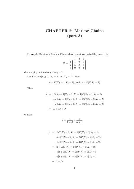
Example Consider a Markov Chain whose transition probability matrix is 

P = 

1 2 3 

1 1 0 0 

2 α β γ 

3 0 0 1 

where α, β, γ > 0 and α + β + γ = 1. 

Let T = min{n ≥ 0 : X n = 1, or X n = 3}. Find 

u = P (X T = 1|X 0 = 2), and v = E(T |X 0 = 2) 

Then 

u = P (X T = 1|X 0 = 2, X 1 = 1)P (X 1 = 1|X 0 = 2) 

+P (X T = 1|X 0 = 2, X 1 = 2)P (X 1 = 2|X 0 = 2) 

+P (X T = 1|X 0 = 2, X 1 = 3)P (X 1 = 3|X 0 = 2) 

= α + uβ + 0γ 

we have 

u = 

α 

1 − β = α 

α + γ 

v = E(T |X 0 = 2, X 1 = 1)P (X 1 = 1|X 0 = 2) 

+E(T |X 0 = 2, X 1 = 2)P (X 1 = 2|X 0 = 2) 

+E(T |X 0 = 2, X 1 = 3)P (X 1 = 3|X 0 = 2) 

= [1 + E(T |X 1 = 1)]P (X 1 = 1|X 0 = 2) 

+[1 + E(T |X 1 = 2)]P (X 1 = 2|X 0 = 2) 

+[1 + E(T |X 1 = 3)]P (X 1 = 3|X 0 = 2) 

= 1 + βv 

1

we have 

v = 1/(1 − β) 

Actually, in this example we can calculate v and u directly. 

Example A Maze A white rat is put into the maze 

1 2 3 

shock 

4 5 6 

7 8 9 

shock 

food 

In the absence of learning, one might hypothesize that the rat would move through the maze 

at random, i.e. if there are k ways to leave a compartment, then the rat would choose each 

of them with equal probability 1/k. Assume that the rat makes one changes to some adjacent 

compartment at each unit of time. Let X n be the compartment occupied at stage n. Suppose 

that compartment 9 contains food and 3 and 7 contain electrical shocking mechanisms. 

1. what is the transition probability matrix 

P = 

1 2 3 4 5 6 7 8 9 

1 0 1/2 0 1/2 0 0 0 0 0 

2 1/3 0 1/3 0 1/3 0 0 0 0 

3 0 0 1 0 0 0 0 0 0 

4 1/3 0 0 0 1/3 0 1/3 0 0 

5 0 1/4 0 1/4 0 1/4 0 1/4 0 

6 0 0 1/3 0 1/3 0 0 0 1/3 

7 0 0 0 0 0 0 1 0 0 

8 0 0 0 0 1/3 0 1/3 0 1/3 

9 0 0 0 0 0 0 0 0 1 

2. If the rat starts in compartment 1, what is the probability that the rate encounters food 

before being shocked. 

Let T = min{n : X n = 3 or X n = 7 or X n = 9}. Let u i = E(X T = 9|X 0 = i), i,e. the 

probability that the rat absorbed by food. Note that there are 3 absorbing states 3, 7 and 

9. It is easy to see that 

u 3 = 0, u 7 = 0, u 9 = 1 

2

we have, for the others i = 1, 2, 4, 5, 6, 8, 

in details 

u i = p i1 u 1 + p i2 u 2 + p i3 u 3 + p i4 u 4 + p i5 u 5 + p i6 u 6 + p i7 u 7 + p i8 u 8 + p i9 u 9 

u 1 = u 0 + u 1 + u 2 + u 3 + u 4 + u 5 + u 6 + u 7 + u 8 

u 2 = u 0 + u 1 + u 2 + u 3 + u 4 + u 5 + u 6 + u 7 + u 8 

u 4 = u 0 + u 1 + u 2 + u 3 + u 4 + u 5 + u 6 + u 7 + u 8 

u 5 = u 0 + u 1 + u 2 + u 3 + u 4 + u 5 + u 6 + u 7 + u 8 

u 6 = u 0 + u 1 + u 2 + u 3 + u 4 + u 5 + u 6 + u 7 + u 8 

u 8 = u 0 + u 1 + u 2 + u 3 + u 4 + u 5 + u 6 + u 7 + u 8 

[PLEASE FILL IN THE COEFFICIENTS] Finally, we have 

u 1 = 0.1429, u 2 = 0.1429, u 2 = 0, u 4 = 0.1429, 

u 5 = 0.2857, u 6 = 0.4286, u 7 = 0, u 8 = 0.4286, u 9 = 1 

3. If the rat starts in compartment 1, how many times it can visit room 5 before it is absorbed? 

Let w i5 = E{ ∑ T −1 

n=0 I(X n = 5)|X 0 = i} we have 

w 15 = p 11 w 15 + p 12 w 25 + p 13 w 35 + p 14 w 45 + p 15 w 55 + p 16 w 65 + p 17 w 75 + p 18 w 85 + p 19 w 95 


w 35 = 0 


w 55 = 1 + p 41 w 15 + p 42 w 25 + p 43 w 35 + p 44 w 45 + p 45 w 55 + p 46 w 65 + p 47 w 75 + p 48 w 85 + p 49 w 95 


w 75 = 0 


w 95 = 0 

or 

w 15 = 0.5w 25 + 0.5w 45 

w 25 = 1 3 w 15 + 1 3 w 35 + 1 3 w 55 

3

w 35 = 0 

w 45 = 1 3 w 15 + 1 3 w 55 + 1 3 w 75 

w 55 = 1 + 1 4 w 25 + 1 4 w 45 + 1 4 w 65 + 1 4 w 85 

w 65 = 1 3 w 35 + 1 3 w 55 + 1 3 w 95 

w 75 = 0 

w 85 = 1 3 w 55 + 1 3 w 75 + 1 3 w 95 

w 95 = 0 

[You can find the answers by solving these set of equations] 

4. If the rat starts in compartment 1, what is the probability that the rat is in 4 before it is 

shocked? 

Let 

z i = P (X T −1 = 4|X 0 = i) 

then 

z 1 = p 12 z 2 + p 14 z 4 

z 2 = p 21 z 1 + p 25 z 5 + p 23 z 3 

z 3 = 0; 

z 4 = p 41 z 1 + p 45 z 5 + p 47 

z 5 = p 52 z 2 + p 54 z 4 + p 56 z 6 + p 58 z 8 

z 6 = p 63 z 3 + p 65 z 5 + p 69 z 9 

z 7 = 0 

z 8 = p 85 z 5 + p 87 0 + p 89 0 

z 9 = 0 

Example A model of Fecundity Changes in sociological patterns such as increase in age at 

marriage, more remarriages after widowhood, and increased divorce rates have profound effects 

on overall population growth rates. Here we attempt to model the life span of a female in a 

population in order to provide a framework for analyzing the effect of social changes on average 

fecundity. 

For a typical woman, we may categorize her in one of the follows states 

E 0 : Prepuberty E 1 : Single E 2 : Married E 3 : Divorced, 

4

E 4 : Widowed 

E 5 : Died or emigration from the population 

Suppose the transition probability matrix is 

P = 

E 0 E 1 E 2 E 3 E 4 E 5 

E 0 0 0.9 0 0 0 0.1 

E 1 0 0.5 0.4 0 0 0.1 

E 2 0 0 0.6 0.2 0.1 0.1 

E 3 0 0 0.4 0.5 0 0.1 

E 4 0 0 0.4 0 0.5 0.1 

E 5 0 0 0 0 0 1 

We are interested in the mean duration spent in state E 2 , Married, since this corresponds to 

the state of maximum fecundity. 

Let w i2 be the mean duration in state E 2 given the initial state is E i . 

From the first step analysis, we have 

w 22 = 1 + p 21 w 12 + p 22 w 22 + p 23 w 32 + p 24 w 42 + p 22 w 52 . 

For absorbing state 5, we have 

w 52 = 0 

If i is not a state 2 and absorbing state 5, 

All together, we have 

w i2 = p i1 w 12 + p i2 w 22 + p i3 w 32 + p i4 w 42 + p i2 w 52 

w 02 = 0w 02 + 0.9w 12 + 0w 22 + 0w 32 + 0.1w 42 + 0.1w 52 

w 12 = w 02 + w 12 + w 22 + w 32 + w 42 + 0w 52 

w 22 = 1 + w 02 + w 12 + w 22 + w 32 + w 42 + 0w 52 

w 32 = w 02 + w 12 + w 22 + w 32 + w 42 + 0w 52 

w 42 = w 02 + w 12 + w 22 + w 32 + w 42 + 0w 52 

w 52 = 0 

The solution is 

w 02 = 4.5, w 12 = 5, w 22 = 6.25, w 32 = 5, w 42 = 5, w 52 = 0. 

Each female, on the average, spend w 02 = 4.5 periods in the childbearing state E 2 during her 

lifetime. 

5

E i . 

Let z i be the proportion of women before she reach E 5 she is single given the initial state is 

z 0 = p 01 z 1 + p 05 0 

z 1 = p 11 z 1 + p 12 z 2 + p 15 1 

z 2 = p 22 z 2 + p 23 z 3 + p 24 z 4 + p 25 0 

z 3 = p 32 z 2 + p 33 z 3 + p 35 0 

z 4 = p 42 z 2 + p 44 z 4 + p 45 0 

z 5 = 0 

we have 

z 0 = 0.0643, z 1 = 0.0714, z 2 = 0, z 3 = 0z 4 = 0, z 5 = 0 

Example [A process with short-term memory, e.g. the weather depends on the past m-days] 

We constrain the weather to two states s: sunny, s: cloudy 

- - - s c s s c s - - 

X n−1 X n X n+1 

Suppose that given the weathers in the previous two days, we can predict the weather in the 

following day as 

sunny (yesterday) + sunny (today) =⇒ sunny (tomorrow) with probability 0.8; 

cloudy (tomorrow) with probability 0.2; 

cloudy (yesterday)+sunny (today) =⇒ sunny (tomorrow) with probability 0.6; 


sunny (yesterday)+cloudy (today) =⇒ sunny (tomorrow) with probability 0.4; 


cloudy (yesterday)+ cloudy (today) =⇒ sunny (tomorrow) with probability 0.1; 


Let X n be the weather of the n’th day. Then the state space is 

S = {s, c} 

6

We have 

P (x n+1 = s|x n−1 = s, x n = s) = 0.8 

P (x n+1 = s|x n−1 = c, x n = s) = 0.6 

Therefore {X t } is not a MC . 

Let Y n = (X n−1 , X n ) be the weather of the day and the previous day. Then the state space 

for {Y n } is 

S = {(s, s), (c, s), (s, c), (c, c)} 

Then {Y t } is a MC with transition probability matrix 

P = 

(s,s) (s,c) (c,s) (c,c) 

(s,s) 0.8 0.2 0 0 

(s,c) 0 0 0.4 0.6 

(c,s) 0.6 0.4 0 0 

(c,c) 0 0 0.1 0.9 

Suppose that in the past two days the weathers are (c, c). In how many days on average can 

we expect to have two successive sunny days? 

To solve the question, we define a new MC by recording the weathers in successive days. 

If there are two successive sunny days, we stop. Denote the process by {Z n }. The transition 

probability matrix is then 

P = 

(s,s) (s,c) (c,s) (c,c) 

(s,s) 1 0 0 0 

(s,c) 0 0 0.4 0.6 

(c,s) 0.6 0.4 0 0 

(c,c) 0 0 0.1 0.9 

Denote the states (s,s), (s, c), (c,s) and (c,c) by 1,2,3 and 4 respectively. Let v i denote the 

expected number of days we first have two sunny days? 

By the first step analysis, we have the following equations 

⎧ 

v 1 = 0 

⎪⎨ 

v 2 = 1 + p 21 v 1 + p 22 v 2 + p 23 v 3 + p 24 v 4 

v ⎪⎩ 3 = 1 + p 31 v 1 + p 32 v 2 + p 33 v 3 + p 34 v 4 

v 4 = 1 + p 41 v 1 + p 42 v 2 + p 43 v 3 + p 44 v 4 

i,e. 

⎧ 

⎪⎨ 

⎪⎩ 

v 1 = 0 

v 2 = 1 + 0.4v 3 + 0.6v 4 

v 3 = 1 + 0.6v 1 + 0.4v 2 

v 4 = 1 + 0.1v 3 + 0.9v 4 

7

we have 

v 2 = 13.3333, v 3 = 6.3333, v 4 = 16.3333 

is 

Example[understanding T] Consider a Markov Chain whose transition probability matrix 

P = 

1 2 3 

1 a b c 

2 d e f 

3 0 0 1 

The MC starts at time 0 with X 0 = 0. Let T = min{n ≥ 0 : X n = 3} Find P (X 3 = 0|X 0 = 

0; T > 3) 

Example [understanding one-step analysis] Consider a Markov Chain whose transition probability 

matrix is 

P = 

The MC starts at time 0 with X0 = 2. 

1 2 3 4 

1 1 0 0 0 

2 0.2 0.2 0.2 0.4 

3 0.2 0.3 0.4 0.1 

4 0 0 0 1 

1. What is the probability that when the process is absorbed, it does so from state 2? 

2. What is the probability that when the process is absorbed by state 4, it does so from state 

2? 

8

CHAPTER 2: Markov Chains (part 3)

Create successful ePaper yourself

Delete template?

Save as template?