discrete-event simulation in clinical trials - Institut für Statistik ...
discrete-event simulation in clinical trials - Institut für Statistik ...
discrete-event simulation in clinical trials - Institut für Statistik ...

Create successful ePaper yourself
Turn your PDF publications into a flip-book with our unique Google optimized e-Paper software.
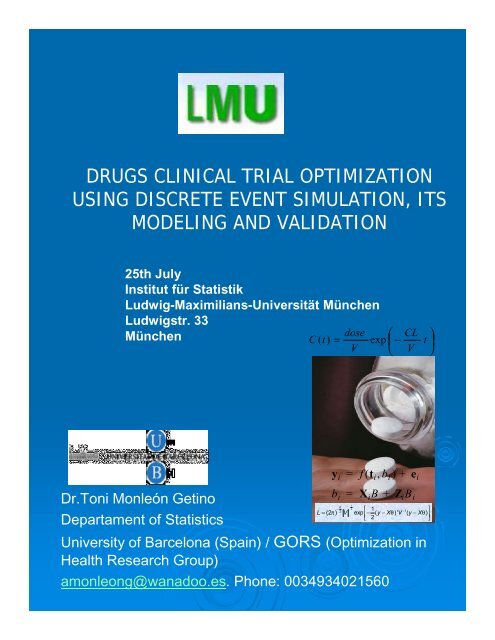
DRUGS CLINICAL TRIAL OPTIMIZATION<br />
USING DISCRETE EVENT SIMULATION, ITS<br />
MODELING AND VALIDATION<br />
25th July<br />
<strong>Institut</strong> <strong>für</strong> <strong>Statistik</strong><br />
Ludwig-Maximilians-Universität München<br />
Ludwigstr. 33<br />
München<br />
dose<br />
⎛ CL ⎞<br />
C ( t)<br />
= exp ⎜ − t ⎟<br />
V ⎝ V ⎠<br />
Dr.Toni Monleón Get<strong>in</strong>o<br />
Departament of Statistics<br />
y = f ( t , b ) + e<br />
i i i i<br />
= X B +<br />
i i i i<br />
University of Barcelona (Spa<strong>in</strong>) / GORS (Optimization <strong>in</strong><br />
Health Research Group)<br />
amonleong@wanadoo.es. Phone: 0034934021560<br />
b<br />
1<br />
n<br />
1<br />
2<br />
ZB<br />
−<br />
− 2<br />
⎡<br />
−1<br />
⎤<br />
L= (2 π) V exp ⎢− ( y − Xθ)' V ( y − Xθ)<br />
⎥<br />
⎣ 2<br />
⎦
ABSTRACT<br />
The possibility of perform<strong>in</strong>g complete <strong>simulation</strong>s of<br />
cl<strong>in</strong>ical <strong>trials</strong>, based on pharmacological action models, has<br />
been considered s<strong>in</strong>ce the advent of the computer era, as<br />
a tool to optimize their practical realisation. Thanks to the<br />
advances <strong>in</strong> computation technology and <strong>in</strong> <strong>discrete</strong> <strong>event</strong><br />
<strong>simulation</strong> tools, today it is possible to perform realistic,<br />
large-scale cl<strong>in</strong>ical trial <strong>simulation</strong>s <strong>in</strong> a regular basis us<strong>in</strong>g<br />
suitable tools of <strong>simulation</strong>.<br />
In this sem<strong>in</strong>ar, we illustrate the process of construct<strong>in</strong>g<br />
realistic <strong>simulation</strong> models based <strong>in</strong> l<strong>in</strong>ear and non-l<strong>in</strong>ear<br />
mixed models us<strong>in</strong>g SAS and the LeanSim framework.<br />
LeanSim is an object-oriented general purpose <strong>simulation</strong><br />
tool, developed <strong>in</strong> C/C++, with a process-<strong>in</strong>teraction<br />
modell<strong>in</strong>g approach. These characteristics of LeanSim<br />
make it very flexible, facilitat<strong>in</strong>g its adaptation to simulate<br />
cl<strong>in</strong>ical <strong>trials</strong>.<br />
Some cl<strong>in</strong>ical <strong>trials</strong> (repeated measures designs) will be<br />
simulated and a methodology to build models of cl<strong>in</strong>ical<br />
<strong>trials</strong> and to simulate, validate and verify statistically them<br />
will be shown. A second part of the talk will be centered <strong>in</strong><br />
the statistical and data analysis facets of model validation<br />
and verification, based on the porcentage variation of<br />
likelihood criteria, compar<strong>in</strong>g the conceptual model and the<br />
<strong>simulation</strong> replications. A last and very <strong>in</strong>complete, for the<br />
moment, part of this research is centered <strong>in</strong> the use of<br />
Bayesian <strong>in</strong>ference to predict the behaviour of drugs <strong>in</strong> the<br />
organism of a new patient, based <strong>in</strong> a population model.<br />
2
Schedule<br />
• Cl<strong>in</strong>ical trial framework<br />
• Modell<strong>in</strong>g and <strong>simulation</strong> of cl<strong>in</strong>ical <strong>trials</strong><br />
• Discrete <strong>event</strong>s <strong>in</strong>tegrated <strong>simulation</strong><br />
• Open questions<br />
3
What is a cl<strong>in</strong>ical trial?<br />
DRUG<br />
Specific effect<br />
Regression to mean<br />
Disease state<br />
Health State<br />
Placebo<br />
Stochastic variations<br />
4
Randomization<br />
5
Cl<strong>in</strong>ical <strong>trials</strong> phases<br />
Phase I: Researchers test a new drug or treatment <strong>in</strong> a small group of<br />
people for the first time to evaluate its safety, determ<strong>in</strong>e a safe dosage range,<br />
and identify side effects.<br />
Phase II: The drug or treatment is given to a larger group of people to see if<br />
it is effective and to further evaluate its safety.<br />
Phase III: The drug or treatment is given to large groups of people to<br />
confirm its effectiveness, monitor side effects, compare it to commonly used<br />
treatments, and collect <strong>in</strong>formation that will allow the drug or treatment to be<br />
used safely.<br />
Phase IV: Studies are done after the drug or treatment has been marketed<br />
to gather <strong>in</strong>formation on the drug's effect <strong>in</strong> various populations and any side<br />
effects associated with long-term use.<br />
6
The bio-pharmacological basis of cl<strong>in</strong>ical <strong>trials</strong><br />
Drug <strong>in</strong> pharmaceutical form<br />
Compartment models<br />
Particle<br />
Periferic compartment (tissues)<br />
Liver<br />
Central compartment<br />
Biological effects<br />
Disolution<br />
dose ⎛ CL ⎞<br />
C ( t)<br />
= exp ⎜ − t ⎟<br />
V ⎝ V ⎠<br />
( t)<br />
= a exp − α t + b exp − β t + c exp − k<br />
( ) ( ) ( t )<br />
C<br />
01<br />
7
The solution of the DE system model will be<br />
discretized and its parametes estimated by means of<br />
NLMM to contemplate population variations with<strong>in</strong><br />
and betwen subjetcs.<br />
8
Dk<br />
k<br />
[ exp( −ket)<br />
− exp( −kat<br />
] ei<br />
e a<br />
C<br />
p<br />
= ) +<br />
Cl(<br />
ka<br />
− ke<br />
)<br />
where<br />
k<br />
a<br />
= exp(0,47 + b )<br />
0i<br />
Cl = exp( − 3,22 + b )<br />
b0i∼N(0; 0,03),<br />
b1i∼N(0;0,4)<br />
eij∼N(0; 0,7).<br />
1i<br />
9
Conceptual Models<br />
PK<br />
e a ( −ket) ( −kat)<br />
Cp<br />
= e − e + ei<br />
Cl( ka<br />
−ke)<br />
⎣<br />
⎦<br />
PD<br />
Dk k<br />
⎡<br />
⎤<br />
% of Movility<br />
85,00<br />
84,50<br />
84,00<br />
83,50<br />
83,00<br />
82,50<br />
82,00<br />
81,50<br />
81,00<br />
80,50<br />
80,00<br />
79,50<br />
79,00<br />
78,50<br />
78,00<br />
Y i = X i b + Z i b i + e i<br />
2 4 6 8 10 12 14<br />
Weeks c s n<br />
Repeated measures models<br />
Phase II-IV<br />
EF<br />
( E<br />
e<br />
max<br />
=<br />
Log ( EC )<br />
+ b1<br />
i)<br />
dosis<br />
50<br />
+ dosis<br />
PK/PD<br />
10
Simulation general<br />
framework
Problem<br />
What if?<br />
Solution?<br />
Model<br />
Simulation<br />
The body<br />
12
Modelization/Simulation process<br />
Statistical analysis (p-value,…)<br />
PK models<br />
2 compartent 1st order model, macro-constants, lagtime,<br />
1st order elim<strong>in</strong>ation<br />
( − α t ) + b exp ( − t ) + c exp ( k t )<br />
C ( t)<br />
= a exp<br />
β −<br />
01<br />
<strong>discrete</strong> approximation of the cont<strong>in</strong>uous differential equations<br />
n replications<br />
Statistical analysis -<br />
<strong>in</strong>ference (p-value,…)<br />
Monte-Carlo<br />
Simulation<br />
y = f ( t , b ) + e<br />
b<br />
i i i i<br />
= X B +<br />
ZB<br />
i i i i<br />
13
Why simulate a CT?<br />
Extrapolate a cl<strong>in</strong>ical trial<br />
Optimize the results<br />
Over parametrized models!<br />
Time extrapolation!<br />
14
Sargent paradigm<br />
15
Validation<br />
‣ The model has been<br />
validated and verified <strong>in</strong><br />
function of a fixed end<br />
po<strong>in</strong>ts (goals).<br />
‣ Sett<strong>in</strong>g end po<strong>in</strong>ts and<br />
establish<strong>in</strong>g the scope<br />
of the model is more<br />
difficult than the<br />
methodology itself.<br />
16
Statistic phases of the process<br />
‣ Validation of the conceptual model:<br />
• Try model<br />
• Parameter estimation or Adjustment<br />
• Validation of the model suppositions:<br />
residual analysis, confidence <strong>in</strong>tervals,<br />
etc<br />
‣ Operational validation: basically<br />
comparation between real data and<br />
simulated data<br />
17
Operational validation<br />
‣ Does the model (conceptual + <strong>simulation</strong>)<br />
reproduces <strong>in</strong> a suitable form the real system?<br />
‣ Usual scope: lihelihood – confidence bands:<br />
goodness of fit<br />
• Null hypothesis: “the model is valid”<br />
• Althernative hypothesis: “The model is wrong”<br />
18
Operational validation:<br />
methodological difficulties<br />
‣ Given an<br />
end po<strong>in</strong>t, a<br />
perfectly<br />
valid model<br />
will be<br />
rejected if<br />
the patient<br />
size (of<br />
<strong>simulation</strong>)<br />
is<br />
sufficiently<br />
big<br />
19
Use of mixed models <strong>in</strong> CTS<br />
‣ Statistical model used<br />
frequently to conceptual<br />
hierarchical (multilevel) of<br />
repeated measures and <strong>in</strong><br />
PK/PD (Proc MIXED /<br />
NLMIXED <strong>in</strong> SAS).<br />
‣ We can model covariance<br />
structure “between” levels and<br />
“with<strong>in</strong>” levels.<br />
‣ We can calculate <strong>in</strong>dividual<br />
trajetories for any patient<br />
20
Mixed model: General form<br />
‣ L<strong>in</strong>ear mixed model form:<br />
Y<br />
i<br />
= X β + Z b + ε<br />
‣ Y i vector of observations<br />
‣ X i y Z i design matrix<br />
‣ β fixed parameters vector<br />
‣ b i ~ N(0,D) random vector of<br />
observations<br />
‣ ε i ~ N(0,Σ i ) residual vector<br />
‣ b i y ε i they are <strong>in</strong>dependent<br />
i<br />
i<br />
i<br />
i<br />
21
Mixed model<br />
‣ L<strong>in</strong>ear mixed model<br />
Y<br />
i<br />
=X β + Z b + ε<br />
i<br />
i<br />
i<br />
i<br />
‣ Fitted to data:<br />
• Parameter estimation<br />
• Parameter CI<br />
• Tests of goodness of fit<br />
22
Types of <strong>simulation</strong>s <strong>in</strong> function of “t”:<br />
Cont<strong>in</strong>ous<br />
Discrete<br />
Discrete <strong>event</strong>s.<br />
The models based on <strong>simulation</strong> of discreet <strong>event</strong>s have sufficient<br />
flexibility and adequacy to the cl<strong>in</strong>ical reality to be used, on the other<br />
way round, the trees of decision and the models of Markov have been<br />
the methods used with major frequency <strong>in</strong> the evaluations<br />
farmacoeconomics, and very rarely <strong>in</strong> the <strong>simulation</strong> of cl<strong>in</strong>ical <strong>trials</strong><br />
(Caro JJ. Pharmacoeconomics 23(4):323-332 2005 ).<br />
Time (t)<br />
General plann<strong>in</strong>g <strong>in</strong> <strong>discrete</strong> time <strong>event</strong>s:<br />
INICIALIZATION<br />
t = 0;<br />
Initialize states of the system and the statistical<br />
counters;<br />
Initialize <strong>event</strong>s list;<br />
PRINCIPAL PROGRAM<br />
If <strong>simulation</strong> time < time rule<br />
Do:<br />
counters;<br />
list;<br />
End;<br />
RESULTS<br />
Determ<strong>in</strong>e type of next <strong>event</strong>;<br />
Advance <strong>simulation</strong> time<br />
Up date condition system + statistical<br />
Generate future <strong>event</strong>s + put <strong>in</strong> the <strong>event</strong><br />
Compute + pr<strong>in</strong>t <strong>in</strong>terest<strong>in</strong>g estimations;<br />
23
Introduction to Discrete Event Simulation<br />
www.dmem.strath.ac.uk/~pball/<strong>simulation</strong>/simulate.html#experimentation<br />
Peter Ball Design Manufacture & Eng<strong>in</strong>eer<strong>in</strong>g Management University of<br />
Strathclyde p.d.ball@strath.ac.uk<br />
SDL->DEVS->PETRI<br />
A <strong>discrete</strong> <strong>event</strong> is someth<strong>in</strong>g that occurs at an <strong>in</strong>stant of time<br />
There are a number of different ways of represent<strong>in</strong>g the logic<br />
with<strong>in</strong> a <strong>discrete</strong> <strong>event</strong> <strong>simulation</strong> model: •Event (patient)<br />
•Activity (Generator, Destroyer, server)<br />
•Process<br />
Detail of the <strong>event</strong> approach structure (from Kreutzer, 1986) 24
SIMULATION METHODOLOGY:<br />
Statistical pakage SAS (SAS <strong>Institut</strong>e, Cary, NC).<br />
LeanSim environment (Guasch y col., 2003)<br />
LEANSIM<br />
New methodology used<br />
complex<br />
environments.<br />
<strong>in</strong><br />
Open and suitable environment.<br />
Discrete <strong>event</strong>s. Library of C+ clases. Class to generate random<br />
multivariate variables bases <strong>in</strong> the method of Jacobi.<br />
Components for manag<strong>in</strong>g <strong>simulation</strong> resources. System of<br />
synchronization between activities and objects. Kernel of <strong>simulation</strong><br />
adapted to support multiple executions. Withdrawal and statistical<br />
analysis of a standard form for all the elements.<br />
Set of classes that allow a representation <strong>in</strong> a three-dimensional<br />
universe.<br />
LeanGen<br />
LeanEditor<br />
LeanStatistics<br />
25
Integrated models and <strong>simulation</strong><br />
Logistics<br />
26
Realistic <strong>simulation</strong> by means of <strong>discrete</strong> envents<br />
Hospital 1<br />
Pacient<br />
…<br />
Hospital n<br />
Total poblation considered<br />
Eligible for the study<br />
Non eligible for the study<br />
Registered on the study<br />
Reflected for the study<br />
Ramdomized<br />
Study treatment assignation<br />
No randomized<br />
Alternativ assignation treatment<br />
Withdrawn<br />
Drop out<br />
Que<strong>in</strong>g dur<strong>in</strong>g visits<br />
Hospital i<br />
T 1<br />
= W(β=2, λ, γ =0)<br />
0 moths<br />
T 2<br />
= fix<br />
2 months+/- 10 days<br />
+/- 10 days<br />
4 months<br />
+/- 10 days<br />
6 months<br />
+/- 10 days<br />
8 meses<br />
Holydays / weekends<br />
N(0, 10)<br />
+/- 10 days<br />
10 months<br />
Time flow<br />
Y ( u n i d a d e s )<br />
Y (unidades)<br />
Riesgo AA<br />
10,3<br />
10,25<br />
10,2<br />
10,15<br />
16<br />
15<br />
14<br />
13<br />
12<br />
11<br />
10<br />
0 2 4 6 8 10<br />
1,2<br />
1<br />
0,8<br />
0,6<br />
0,4<br />
0,2<br />
Pacebo (Conceptual)<br />
10,1<br />
0 2 4 6 8 10<br />
Pacebo (Conceptual)<br />
50 mg (Conceptual)<br />
100 mg (Conceptual)<br />
Placebo (Conceptual)<br />
50 mg (Conceptual)<br />
Modelo de enfermedad<br />
Tiempo (meses)<br />
100 mg (Conceptual)<br />
Atribute variation<br />
Modelo de enfermedad<br />
Tiempo (meses)<br />
0<br />
0 5 10 15 20 25<br />
Tiempo (meses)<br />
Dosis de máximo efecto<br />
Dosis óptima<br />
Complete cl<strong>in</strong>ical trial<br />
Models<br />
Simulation:<br />
•Var between-patients,<br />
•Var <strong>in</strong>ter-patient<br />
•Global error<br />
Disease sub-model<br />
Efficacy<br />
submodel<br />
Safety submodel<br />
27
EXAMPLE OF MODELLING AND SIMULATION OF PHASE II-III<br />
CLINICAL TRIAL BASED IN DRUG ACTION AND DISEASE<br />
MODEL<br />
‣N=144 patients (40 per dos<strong>in</strong>g group (+ withdrawn):<br />
placebo, 50 mg or 100 mg). α=0,05 y β=0,80; δ = 3,2 (Y)<br />
‣End po<strong>in</strong>t: Search<strong>in</strong>g the most efficient dose to treat<br />
disease (E), but m<strong>in</strong>imiz<strong>in</strong>g the risk of adverse <strong>event</strong>s (side<br />
effects).<br />
‣ p-value treatments < 0,05<br />
‣ p-valor adverse <strong>event</strong>s < 0,05<br />
‣Scope of the <strong>simulation</strong>:<br />
Pharmacological action (PD).<br />
Disease model (E)<br />
Use of different parameters PK/PD of previous cl<strong>in</strong>ical<br />
<strong>trials</strong> (Fase I).<br />
Efficacy.<br />
Safety.<br />
Logistic subjects (number of hospitals recuit<strong>in</strong>g<br />
patients, recuit<strong>in</strong>g time, time between visits, time of last<br />
visit (end of cl<strong>in</strong>ical trial) withdrawn, etc).<br />
‣Time schedule: 11 visits, every moth (0,1,2,…, 10 months).<br />
‣First end po<strong>in</strong>t: Y (efficacy), RAA (Safety): Risk of adverse<br />
<strong>event</strong>.<br />
28
STATISTICAL MODELLING<br />
1-Disease progress:<br />
E = 10+ 0,1( b + slope )<br />
0i<br />
b 0i ∼N(0; 1)<br />
slope = oscillations of the disease<br />
<strong>in</strong> the time = 2<br />
2-Effect of the drug over Y (Efficacy):<br />
EF<br />
( E<br />
e<br />
max<br />
=<br />
Log ( EC )<br />
+ b1<br />
i)<br />
dosis<br />
50<br />
+ dosis<br />
EF = drug effect<br />
b 1i ∼N(0; 1) E max = 0,5<br />
Log(EC50) = 1,5 (100mg); 4,5 (50 mg)<br />
Y = E *(1 + EF * RAF)<br />
+<br />
e ij ∼N(0, 2).<br />
e i<br />
Sub-models<br />
RAF<br />
= 1−<br />
e<br />
−RATE*<br />
tiempo<br />
RAF = effect of the time delay<br />
on the drug action<br />
RATE = 0,5<br />
3-Adverse <strong>event</strong> risk (Stanski y Jenk<strong>in</strong>s,2004) (Safety):<br />
RAA<br />
e<br />
1+<br />
e<br />
( −k<br />
+ ( c+<br />
b<br />
1i<br />
=<br />
( −k<br />
+ ( c+<br />
b<br />
)* tiempo)<br />
1i<br />
)* tiempo)<br />
+ e<br />
K = moment of rise AA<br />
c = 0,11 (placebo), 0,35 (50 mg) y 0,45 (100 mg).<br />
b 1i ∼N(0; 0,01) e ij ∼N(0; 0,1).<br />
i<br />
4-Logistic characteristics-> Integrated model<br />
•Withdrawns: 20% (5% per visit)<br />
•Stochastic distribution of patients recruitement ∼ Weibull<br />
•Error time dur<strong>in</strong>g the visit ∼ Normal<br />
•Behaviour of hopitals dur<strong>in</strong>g recruitement (same number of<br />
patients / time delay)<br />
29
CONCEPTUAL MODEL SIMULATION (Plann<strong>in</strong>g)<br />
Generator<br />
N=144<br />
W(β=2, δ, γ=0)<br />
W 1<br />
W<br />
δ =10<br />
2 W 3<br />
δ =15 δ =20<br />
HOSPITAL 1<br />
HOSPITAL 2<br />
HOSPITAL 3<br />
n=6 visits<br />
W i<br />
+ t j<br />
+ N(0, 10) [t = time between visits]<br />
Wait<strong>in</strong>g<br />
Server<br />
p withdrawn<br />
=0,03<br />
.<br />
.<br />
.<br />
10,3<br />
.<br />
.<br />
.<br />
Change <strong>in</strong> attributes<br />
Pacebo (Conceptual)<br />
Destructor:<br />
End<br />
Destructor:<br />
Withdrawn<br />
Y (unidades)<br />
10,25<br />
10,2<br />
10,15<br />
Modelo de enfermedad<br />
Placebo<br />
10,1<br />
0 2 4 6 8 10<br />
Tiempo (meses)<br />
Treatment<br />
assignation<br />
50 mg<br />
100 mg<br />
Y (unidades)<br />
16<br />
15<br />
14<br />
13<br />
12<br />
11<br />
Pacebo (Conceptual)<br />
50 mg (Conceptual) Dosis de máximo efecto<br />
100 mg (Conceptual)<br />
Dosis óptima<br />
Modelo de enfermedad<br />
10<br />
0 2 4 6 8 10<br />
Tiempo (meses)<br />
Riesgo AA<br />
1,2<br />
1<br />
0,8<br />
0,6<br />
0,4<br />
Placebo (Conceptual)<br />
50 mg (Conceptual)<br />
100 mg (Conceptual)<br />
0,2<br />
0<br />
0 5 10 15 20 25<br />
Tiempo (meses)<br />
30
N=144<br />
Start of CT<br />
W(10)<br />
0 months<br />
Time<br />
Hospital 1<br />
Generator<br />
48 patients<br />
48 patients<br />
48 patients<br />
Hospital 2<br />
+/- 10 days<br />
2 monts 0 months<br />
+/- 10 days 2 months<br />
4 months<br />
+/- 10 days<br />
4 months<br />
6 months<br />
+/- 10 days<br />
8 months<br />
+/- 10 days<br />
10 months<br />
Time<br />
W(15) W(20)<br />
6 months<br />
8 months<br />
Recruit<strong>in</strong>g delay TIME<br />
Hospital 3<br />
0 months<br />
2 months<br />
4 months<br />
Time<br />
6 months<br />
8 months<br />
End CT<br />
10 months<br />
10 months<br />
ECT = TR + TBV (fix) + TEBV + Que<strong>in</strong>g + Calendar + Withdrawns<br />
Que<strong>in</strong>g (restrictions)<br />
Calendars (Hollidays, …)<br />
31
Variation <strong>in</strong> cl<strong>in</strong>ical end po<strong>in</strong>ts<br />
Efficacy submodel<br />
16<br />
Placebo (Conceptual) 50 mg (Conceptual)<br />
100 mg (Conceptual) Placebo (Simulación)<br />
50 mg (Simulación) 100 mg Simulación<br />
Risk AA Y (unities)<br />
Y (unidades)<br />
Riesgo AA<br />
15<br />
14<br />
13<br />
12<br />
11<br />
10<br />
PVMCBV:<br />
1<br />
0,8<br />
0,6<br />
0,4<br />
0,2<br />
0 2 4 6 8 10<br />
Time (months)<br />
Tiempo (meses)<br />
p= 0,0466 [-0,01136; 0,10472],<br />
VMCBP:<br />
0<br />
λ : 0,78 a un 12%<br />
Safety sub-model<br />
Placebo (Conceptual) 50 mg (Conceptual)<br />
100 mg (Conceptual) Placebo (Simulación)<br />
50 mg (Simulación) 100 mg (Simulación)<br />
0<br />
0 2 4 6 8 10<br />
Tiempo (meses)<br />
Time (months)<br />
0<br />
PVMCBV: p= 0,0230 [-0,0208; 0,06699]<br />
32
Determ<strong>in</strong>ation of the end<strong>in</strong>g moment of the CT:<br />
The ed<strong>in</strong>g moment CT have calculated (Day 0 a Visit 10 month) per<br />
hospital, us<strong>in</strong>g 40 <strong>simulation</strong> replications:<br />
•Hospital 1: 385,525 [381,132; 389,917] days<br />
•Hospital 2: 385,975 [381,169; 390,780] days<br />
•Hospital 3: 393,575 [388,773; 398,376] days<br />
8<br />
7<br />
6<br />
5<br />
4<br />
3<br />
2<br />
1<br />
0<br />
Centro 1<br />
Centro 2<br />
Centro 3<br />
234<br />
264<br />
275<br />
280<br />
287<br />
292<br />
297<br />
302<br />
308<br />
315<br />
321<br />
326<br />
331<br />
336<br />
343<br />
350<br />
363<br />
374<br />
399<br />
Duration od the Cl<strong>in</strong>ical trial(days)<br />
Duración del ensayo clínico (días)<br />
Simulation scenarios:<br />
1- Increase 50 % the speed of recruitment respect regard to the <strong>in</strong>itial<br />
model:<br />
•Hospital 1: 381,125 [375,822; 386,427] días<br />
•Hospital 2: 387,475 [381,271; 317,222] días<br />
•Hospital 3: 391,075 [386,617; 395,532] días<br />
2-The recruitment period for the 3 hopitals has been changed for 90<br />
days average:<br />
•Hospital 1: 531,414 [519,611; 543,217] días<br />
•Hospital 2: 532,829 [522,036; 543,622] días<br />
•Hospital 3: 535,780 [525,433; 546,127] días<br />
33
Open questions<br />
‣ Prediction of a new trajectory for a new case<br />
(imcomplete) us<strong>in</strong>g the population <strong>in</strong>formation <strong>in</strong> PK<br />
(Bayesian prediction)<br />
Interest<strong>in</strong>g<br />
implications <strong>in</strong> adjust<br />
the drug dose to the<br />
patient, m<strong>in</strong>imize risk<br />
of toxicity, <strong>in</strong>crease<br />
efficacy<br />
Prior<br />
Posterior<br />
SAS<br />
34
‣Validation/Verification methodologies for<br />
complex <strong>simulation</strong> models<br />
C oncentración (m g/L)<br />
12<br />
10<br />
8<br />
6<br />
4<br />
2<br />
0<br />
0 2 4 6 8 10 12 14 16 18 20 22 24<br />
Tiempo (h)<br />
Conceptual<br />
Conceptual model<br />
Concentración Real data real<br />
Concentración (mg/L)<br />
12<br />
10<br />
8<br />
6<br />
4<br />
2<br />
Simulation model (IC95%)<br />
0<br />
0 2 4 6 8 10 12 14 16 18 20 22 24<br />
Tiempo (h)<br />
Simulation<br />
Simulación Conceptual<br />
PVLIR<br />
i<br />
LLR − LLRi<br />
100<br />
LLR<br />
=<br />
2<br />
2<br />
35
1<br />
n<br />
1<br />
2<br />
−<br />
− 2<br />
⎡<br />
−1<br />
⎤<br />
L= (2 π) V exp ⎢− ( y −Xθ)' V ( y −Xθ)<br />
⎥<br />
⎣ 2<br />
⎦<br />
%-LL<br />
12<br />
C<br />
C<br />
11 C<br />
C<br />
C<br />
C<br />
C<br />
C<br />
CC<br />
C<br />
C<br />
C<br />
C<br />
10<br />
C<br />
C C<br />
C<br />
C C<br />
C<br />
C C<br />
C<br />
C<br />
C<br />
C C C<br />
C C C<br />
C C C C<br />
C C<br />
C C C<br />
C C<br />
C<br />
CC<br />
C C<br />
C C C<br />
CC<br />
CC<br />
C<br />
C C<br />
C<br />
CC<br />
C C<br />
C<br />
9<br />
C<br />
CC<br />
C C C<br />
C C<br />
C<br />
C C<br />
C<br />
C<br />
C<br />
C<br />
C<br />
CC<br />
8<br />
C C<br />
CC<br />
CC<br />
C C<br />
C C<br />
CC<br />
C<br />
C<br />
C<br />
C C<br />
CC<br />
C C<br />
C<br />
C C<br />
C C<br />
C C C<br />
C<br />
C<br />
C<br />
C<br />
C<br />
7<br />
C C<br />
C<br />
C<br />
C<br />
C<br />
C C<br />
C<br />
C<br />
C<br />
C C<br />
C C C<br />
C C<br />
C C<br />
C C<br />
C<br />
C<br />
CC<br />
C C C<br />
C<br />
C<br />
C<br />
C C<br />
C C C<br />
C<br />
C<br />
C<br />
C C<br />
C<br />
C<br />
C<br />
C<br />
C<br />
C<br />
C<br />
C<br />
C<br />
C<br />
C C<br />
C<br />
C<br />
C<br />
C C<br />
C CC C C<br />
C C<br />
C<br />
C<br />
C<br />
C C<br />
C<br />
C<br />
C<br />
C<br />
C<br />
C 6<br />
C<br />
C<br />
C<br />
C<br />
CC<br />
C C<br />
C<br />
C<br />
C C<br />
C<br />
C<br />
C C<br />
C<br />
C<br />
C C<br />
C<br />
CC<br />
C<br />
C C<br />
C<br />
C C<br />
C<br />
C<br />
C<br />
C<br />
C<br />
CC<br />
C<br />
C<br />
C<br />
C<br />
C C<br />
C<br />
C<br />
C C<br />
C C<br />
C<br />
C<br />
C C<br />
C<br />
C C<br />
C<br />
C<br />
C<br />
C C C C<br />
CC<br />
CC<br />
C<br />
C C<br />
CC C<br />
C<br />
C<br />
C C C<br />
C<br />
C C<br />
C<br />
C<br />
C<br />
CC<br />
C C<br />
C<br />
C C<br />
C<br />
C C<br />
C<br />
C C C<br />
C C<br />
C<br />
C<br />
C<br />
C C<br />
C<br />
C C<br />
C<br />
C C<br />
C<br />
C<br />
C C<br />
CC<br />
C C<br />
C C C<br />
C<br />
C<br />
C<br />
C<br />
CC<br />
C<br />
C<br />
C C<br />
C<br />
C C<br />
C C<br />
C<br />
C<br />
C C<br />
C<br />
C<br />
C C<br />
C<br />
C<br />
C<br />
C<br />
C<br />
C C<br />
C C C<br />
C<br />
5<br />
C<br />
C<br />
C C<br />
C<br />
C C<br />
C C C<br />
C<br />
C C<br />
C<br />
CC<br />
C C<br />
C<br />
C<br />
C<br />
C<br />
C C<br />
C<br />
C C<br />
C<br />
C<br />
C C C<br />
C C<br />
C<br />
C<br />
C<br />
C C C<br />
C C<br />
C<br />
C C C<br />
C<br />
C<br />
C C C C C<br />
C<br />
C<br />
C<br />
C<br />
C<br />
C C<br />
C C<br />
C<br />
C<br />
C<br />
C<br />
C C<br />
C C C<br />
C<br />
C<br />
4 C<br />
C<br />
C<br />
C C<br />
C C<br />
C<br />
C C C<br />
C<br />
C C<br />
C<br />
C<br />
C<br />
C C<br />
C<br />
C C C C C<br />
C C<br />
C<br />
C<br />
C<br />
C<br />
C<br />
C<br />
C<br />
C<br />
C C<br />
C<br />
C<br />
3<br />
C<br />
C<br />
C<br />
C<br />
C<br />
2<br />
C<br />
0 100 200 300 400 500 600 700 800 900 1000<br />
Number of replications<br />
PLOT %-LL %AIC %AIC CCC%AIC<br />
Percentage of PVL between 1000 <strong>simulation</strong> replicas and conceptual model us<strong>in</strong>g the<br />
computacional model (σ= 2,8532) (Range:2.44379-11.8056 for BIC, 2.19090-<br />
11.56709 for AICC, 2.18605- 11.56225 for AIC, 2.09318-11.49733 for -LLR ).<br />
%-LL<br />
35<br />
C<br />
34<br />
C<br />
C<br />
C<br />
C C<br />
33<br />
C<br />
C<br />
C<br />
C<br />
C<br />
C<br />
C<br />
32 C<br />
C C<br />
C CC<br />
C C<br />
C<br />
CC<br />
C C<br />
C C<br />
C<br />
C CC<br />
C C<br />
C<br />
C<br />
C<br />
C C<br />
C<br />
C CC<br />
CC<br />
C<br />
C<br />
C<br />
C<br />
C<br />
C C<br />
C<br />
31<br />
C<br />
CC<br />
CC C<br />
C<br />
C<br />
C<br />
C<br />
C<br />
C<br />
C<br />
C<br />
C<br />
C C<br />
C<br />
C<br />
C<br />
30<br />
C<br />
C C<br />
C<br />
C<br />
C<br />
C<br />
C C C<br />
C C<br />
C C<br />
C<br />
C C C<br />
C<br />
C<br />
C<br />
C<br />
C<br />
C C<br />
CC<br />
C<br />
C<br />
C<br />
C C<br />
C<br />
C<br />
C C C C<br />
C<br />
C<br />
C C<br />
C<br />
C<br />
C C C C<br />
C<br />
C<br />
C<br />
C<br />
C<br />
29<br />
C<br />
C C<br />
C<br />
C C<br />
C C<br />
C<br />
C<br />
C<br />
C<br />
C<br />
C<br />
C<br />
C C<br />
C<br />
C<br />
C C C C<br />
C<br />
C<br />
C<br />
C<br />
CC<br />
C<br />
C<br />
C C C<br />
C<br />
28 C<br />
C<br />
C<br />
C<br />
C<br />
C<br />
C<br />
C C<br />
C C C<br />
C<br />
CC<br />
C<br />
C<br />
C C<br />
C C<br />
C<br />
C<br />
C<br />
C<br />
C<br />
C<br />
C<br />
C C<br />
C<br />
C<br />
C<br />
CC<br />
C<br />
C C<br />
C C<br />
C C<br />
CC<br />
C<br />
C<br />
C<br />
C<br />
C C<br />
C<br />
CC<br />
C<br />
C<br />
C<br />
C C<br />
C<br />
CC C<br />
C<br />
C C<br />
C CC<br />
C<br />
CC<br />
C<br />
C<br />
C<br />
C<br />
CC<br />
C CC<br />
C<br />
C C CC C<br />
C<br />
C<br />
C<br />
C<br />
C<br />
C<br />
C C C<br />
C<br />
C CC<br />
C<br />
C C<br />
C<br />
C C<br />
C<br />
27<br />
C<br />
C<br />
C<br />
C C<br />
C<br />
C<br />
C C<br />
C<br />
CC<br />
C<br />
CC<br />
C<br />
C<br />
CC<br />
C C C C<br />
C<br />
C<br />
C<br />
C<br />
C C<br />
C<br />
C<br />
C<br />
C<br />
C<br />
C<br />
C<br />
C CC<br />
CC<br />
C<br />
C<br />
C C C<br />
C<br />
C<br />
C C C<br />
C C C C<br />
C<br />
C C C<br />
C<br />
C<br />
CC<br />
C<br />
C<br />
C<br />
C<br />
C<br />
C<br />
C<br />
C C C CC C<br />
C<br />
C C<br />
C<br />
C C<br />
C<br />
C<br />
C<br />
C<br />
C<br />
C<br />
C<br />
C C C C C<br />
C<br />
C<br />
C<br />
CC<br />
C C C<br />
C<br />
C C<br />
C C C C<br />
C C<br />
C<br />
C<br />
C<br />
C<br />
C<br />
C<br />
C C C<br />
C<br />
C C C C<br />
C C<br />
C<br />
C<br />
CC<br />
C<br />
C<br />
C<br />
CC<br />
C C C<br />
C C C<br />
26 C C CC<br />
C<br />
C C<br />
C<br />
C C C C<br />
C C C C<br />
C C<br />
C<br />
C CC<br />
C<br />
C<br />
C<br />
C<br />
C<br />
C<br />
C<br />
C<br />
C<br />
25<br />
C C<br />
C C<br />
C<br />
C<br />
C<br />
C<br />
24<br />
σ<br />
0 100 200 300 400 500 600 700 800 900 1000<br />
Number of replications<br />
PLOT %-LL %AIC %AIC CCC%AIC<br />
Percentage of PVL between 1000 <strong>simulation</strong> replicas and conceptual model <strong>in</strong>creas<strong>in</strong>g<br />
the variability of the global model error (σ=5) <strong>in</strong> the upper range (Range: 23.9939-<br />
33.9592 for BIC, 24.2873- 34.2680 for AICC, 24.2922- 34.2729 for AIC, 24.4640 -<br />
34.4744 for -LLR )<br />
36
Vielen dank <strong>für</strong><br />
Ihre<br />
Aufmerksamkeit<br />
37