discrete-event simulation in clinical trials - Institut für Statistik ...
discrete-event simulation in clinical trials - Institut für Statistik ...
discrete-event simulation in clinical trials - Institut für Statistik ...

You also want an ePaper? Increase the reach of your titles
YUMPU automatically turns print PDFs into web optimized ePapers that Google loves.
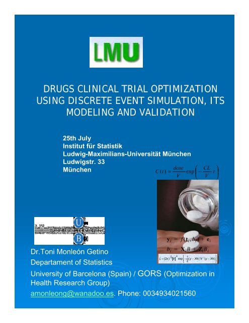
DRUGS CLINICAL TRIAL OPTIMIZATION<br />
USING DISCRETE EVENT SIMULATION, ITS<br />
MODELING AND VALIDATION<br />
25th July<br />
<strong>Institut</strong> <strong>für</strong> <strong>Statistik</strong><br />
Ludwig-Maximilians-Universität München<br />
Ludwigstr. 33<br />
München<br />
dose<br />
⎛ CL ⎞<br />
C ( t)<br />
= exp ⎜ − t ⎟<br />
V ⎝ V ⎠<br />
Dr.Toni Monleón Get<strong>in</strong>o<br />
Departament of Statistics<br />
y = f ( t , b ) + e<br />
i i i i<br />
= X B +<br />
i i i i<br />
University of Barcelona (Spa<strong>in</strong>) / GORS (Optimization <strong>in</strong><br />
Health Research Group)<br />
amonleong@wanadoo.es. Phone: 0034934021560<br />
b<br />
1<br />
n<br />
1<br />
2<br />
ZB<br />
−<br />
− 2<br />
⎡<br />
−1<br />
⎤<br />
L= (2 π) V exp ⎢− ( y − Xθ)' V ( y − Xθ)<br />
⎥<br />
⎣ 2<br />
⎦
ABSTRACT<br />
The possibility of perform<strong>in</strong>g complete <strong>simulation</strong>s of<br />
cl<strong>in</strong>ical <strong>trials</strong>, based on pharmacological action models, has<br />
been considered s<strong>in</strong>ce the advent of the computer era, as<br />
a tool to optimize their practical realisation. Thanks to the<br />
advances <strong>in</strong> computation technology and <strong>in</strong> <strong>discrete</strong> <strong>event</strong><br />
<strong>simulation</strong> tools, today it is possible to perform realistic,<br />
large-scale cl<strong>in</strong>ical trial <strong>simulation</strong>s <strong>in</strong> a regular basis us<strong>in</strong>g<br />
suitable tools of <strong>simulation</strong>.<br />
In this sem<strong>in</strong>ar, we illustrate the process of construct<strong>in</strong>g<br />
realistic <strong>simulation</strong> models based <strong>in</strong> l<strong>in</strong>ear and non-l<strong>in</strong>ear<br />
mixed models us<strong>in</strong>g SAS and the LeanSim framework.<br />
LeanSim is an object-oriented general purpose <strong>simulation</strong><br />
tool, developed <strong>in</strong> C/C++, with a process-<strong>in</strong>teraction<br />
modell<strong>in</strong>g approach. These characteristics of LeanSim<br />
make it very flexible, facilitat<strong>in</strong>g its adaptation to simulate<br />
cl<strong>in</strong>ical <strong>trials</strong>.<br />
Some cl<strong>in</strong>ical <strong>trials</strong> (repeated measures designs) will be<br />
simulated and a methodology to build models of cl<strong>in</strong>ical<br />
<strong>trials</strong> and to simulate, validate and verify statistically them<br />
will be shown. A second part of the talk will be centered <strong>in</strong><br />
the statistical and data analysis facets of model validation<br />
and verification, based on the porcentage variation of<br />
likelihood criteria, compar<strong>in</strong>g the conceptual model and the<br />
<strong>simulation</strong> replications. A last and very <strong>in</strong>complete, for the<br />
moment, part of this research is centered <strong>in</strong> the use of<br />
Bayesian <strong>in</strong>ference to predict the behaviour of drugs <strong>in</strong> the<br />
organism of a new patient, based <strong>in</strong> a population model.<br />
2
Schedule<br />
• Cl<strong>in</strong>ical trial framework<br />
• Modell<strong>in</strong>g and <strong>simulation</strong> of cl<strong>in</strong>ical <strong>trials</strong><br />
• Discrete <strong>event</strong>s <strong>in</strong>tegrated <strong>simulation</strong><br />
• Open questions<br />
3
What is a cl<strong>in</strong>ical trial?<br />
DRUG<br />
Specific effect<br />
Regression to mean<br />
Disease state<br />
Health State<br />
Placebo<br />
Stochastic variations<br />
4
Randomization<br />
5
Cl<strong>in</strong>ical <strong>trials</strong> phases<br />
Phase I: Researchers test a new drug or treatment <strong>in</strong> a small group of<br />
people for the first time to evaluate its safety, determ<strong>in</strong>e a safe dosage range,<br />
and identify side effects.<br />
Phase II: The drug or treatment is given to a larger group of people to see if<br />
it is effective and to further evaluate its safety.<br />
Phase III: The drug or treatment is given to large groups of people to<br />
confirm its effectiveness, monitor side effects, compare it to commonly used<br />
treatments, and collect <strong>in</strong>formation that will allow the drug or treatment to be<br />
used safely.<br />
Phase IV: Studies are done after the drug or treatment has been marketed<br />
to gather <strong>in</strong>formation on the drug's effect <strong>in</strong> various populations and any side<br />
effects associated with long-term use.<br />
6
The bio-pharmacological basis of cl<strong>in</strong>ical <strong>trials</strong><br />
Drug <strong>in</strong> pharmaceutical form<br />
Compartment models<br />
Particle<br />
Periferic compartment (tissues)<br />
Liver<br />
Central compartment<br />
Biological effects<br />
Disolution<br />
dose ⎛ CL ⎞<br />
C ( t)<br />
= exp ⎜ − t ⎟<br />
V ⎝ V ⎠<br />
( t)<br />
= a exp − α t + b exp − β t + c exp − k<br />
( ) ( ) ( t )<br />
C<br />
01<br />
7
The solution of the DE system model will be<br />
discretized and its parametes estimated by means of<br />
NLMM to contemplate population variations with<strong>in</strong><br />
and betwen subjetcs.<br />
8
Dk<br />
k<br />
[ exp( −ket)<br />
− exp( −kat<br />
] ei<br />
e a<br />
C<br />
p<br />
= ) +<br />
Cl(<br />
ka<br />
− ke<br />
)<br />
where<br />
k<br />
a<br />
= exp(0,47 + b )<br />
0i<br />
Cl = exp( − 3,22 + b )<br />
b0i∼N(0; 0,03),<br />
b1i∼N(0;0,4)<br />
eij∼N(0; 0,7).<br />
1i<br />
9
Conceptual Models<br />
PK<br />
e a ( −ket) ( −kat)<br />
Cp<br />
= e − e + ei<br />
Cl( ka<br />
−ke)<br />
⎣<br />
⎦<br />
PD<br />
Dk k<br />
⎡<br />
⎤<br />
% of Movility<br />
85,00<br />
84,50<br />
84,00<br />
83,50<br />
83,00<br />
82,50<br />
82,00<br />
81,50<br />
81,00<br />
80,50<br />
80,00<br />
79,50<br />
79,00<br />
78,50<br />
78,00<br />
Y i = X i b + Z i b i + e i<br />
2 4 6 8 10 12 14<br />
Weeks c s n<br />
Repeated measures models<br />
Phase II-IV<br />
EF<br />
( E<br />
e<br />
max<br />
=<br />
Log ( EC )<br />
+ b1<br />
i)<br />
dosis<br />
50<br />
+ dosis<br />
PK/PD<br />
10
Simulation general<br />
framework
Problem<br />
What if?<br />
Solution?<br />
Model<br />
Simulation<br />
The body<br />
12
Modelization/Simulation process<br />
Statistical analysis (p-value,…)<br />
PK models<br />
2 compartent 1st order model, macro-constants, lagtime,<br />
1st order elim<strong>in</strong>ation<br />
( − α t ) + b exp ( − t ) + c exp ( k t )<br />
C ( t)<br />
= a exp<br />
β −<br />
01<br />
<strong>discrete</strong> approximation of the cont<strong>in</strong>uous differential equations<br />
n replications<br />
Statistical analysis -<br />
<strong>in</strong>ference (p-value,…)<br />
Monte-Carlo<br />
Simulation<br />
y = f ( t , b ) + e<br />
b<br />
i i i i<br />
= X B +<br />
ZB<br />
i i i i<br />
13
Why simulate a CT?<br />
Extrapolate a cl<strong>in</strong>ical trial<br />
Optimize the results<br />
Over parametrized models!<br />
Time extrapolation!<br />
14
Sargent paradigm<br />
15
Validation<br />
‣ The model has been<br />
validated and verified <strong>in</strong><br />
function of a fixed end<br />
po<strong>in</strong>ts (goals).<br />
‣ Sett<strong>in</strong>g end po<strong>in</strong>ts and<br />
establish<strong>in</strong>g the scope<br />
of the model is more<br />
difficult than the<br />
methodology itself.<br />
16
Statistic phases of the process<br />
‣ Validation of the conceptual model:<br />
• Try model<br />
• Parameter estimation or Adjustment<br />
• Validation of the model suppositions:<br />
residual analysis, confidence <strong>in</strong>tervals,<br />
etc<br />
‣ Operational validation: basically<br />
comparation between real data and<br />
simulated data<br />
17
Operational validation<br />
‣ Does the model (conceptual + <strong>simulation</strong>)<br />
reproduces <strong>in</strong> a suitable form the real system?<br />
‣ Usual scope: lihelihood – confidence bands:<br />
goodness of fit<br />
• Null hypothesis: “the model is valid”<br />
• Althernative hypothesis: “The model is wrong”<br />
18
Operational validation:<br />
methodological difficulties<br />
‣ Given an<br />
end po<strong>in</strong>t, a<br />
perfectly<br />
valid model<br />
will be<br />
rejected if<br />
the patient<br />
size (of<br />
<strong>simulation</strong>)<br />
is<br />
sufficiently<br />
big<br />
19
Use of mixed models <strong>in</strong> CTS<br />
‣ Statistical model used<br />
frequently to conceptual<br />
hierarchical (multilevel) of<br />
repeated measures and <strong>in</strong><br />
PK/PD (Proc MIXED /<br />
NLMIXED <strong>in</strong> SAS).<br />
‣ We can model covariance<br />
structure “between” levels and<br />
“with<strong>in</strong>” levels.<br />
‣ We can calculate <strong>in</strong>dividual<br />
trajetories for any patient<br />
20
Mixed model: General form<br />
‣ L<strong>in</strong>ear mixed model form:<br />
Y<br />
i<br />
= X β + Z b + ε<br />
‣ Y i vector of observations<br />
‣ X i y Z i design matrix<br />
‣ β fixed parameters vector<br />
‣ b i ~ N(0,D) random vector of<br />
observations<br />
‣ ε i ~ N(0,Σ i ) residual vector<br />
‣ b i y ε i they are <strong>in</strong>dependent<br />
i<br />
i<br />
i<br />
i<br />
21
Mixed model<br />
‣ L<strong>in</strong>ear mixed model<br />
Y<br />
i<br />
=X β + Z b + ε<br />
i<br />
i<br />
i<br />
i<br />
‣ Fitted to data:<br />
• Parameter estimation<br />
• Parameter CI<br />
• Tests of goodness of fit<br />
22
Types of <strong>simulation</strong>s <strong>in</strong> function of “t”:<br />
Cont<strong>in</strong>ous<br />
Discrete<br />
Discrete <strong>event</strong>s.<br />
The models based on <strong>simulation</strong> of discreet <strong>event</strong>s have sufficient<br />
flexibility and adequacy to the cl<strong>in</strong>ical reality to be used, on the other<br />
way round, the trees of decision and the models of Markov have been<br />
the methods used with major frequency <strong>in</strong> the evaluations<br />
farmacoeconomics, and very rarely <strong>in</strong> the <strong>simulation</strong> of cl<strong>in</strong>ical <strong>trials</strong><br />
(Caro JJ. Pharmacoeconomics 23(4):323-332 2005 ).<br />
Time (t)<br />
General plann<strong>in</strong>g <strong>in</strong> <strong>discrete</strong> time <strong>event</strong>s:<br />
INICIALIZATION<br />
t = 0;<br />
Initialize states of the system and the statistical<br />
counters;<br />
Initialize <strong>event</strong>s list;<br />
PRINCIPAL PROGRAM<br />
If <strong>simulation</strong> time < time rule<br />
Do:<br />
counters;<br />
list;<br />
End;<br />
RESULTS<br />
Determ<strong>in</strong>e type of next <strong>event</strong>;<br />
Advance <strong>simulation</strong> time<br />
Up date condition system + statistical<br />
Generate future <strong>event</strong>s + put <strong>in</strong> the <strong>event</strong><br />
Compute + pr<strong>in</strong>t <strong>in</strong>terest<strong>in</strong>g estimations;<br />
23
Introduction to Discrete Event Simulation<br />
www.dmem.strath.ac.uk/~pball/<strong>simulation</strong>/simulate.html#experimentation<br />
Peter Ball Design Manufacture & Eng<strong>in</strong>eer<strong>in</strong>g Management University of<br />
Strathclyde p.d.ball@strath.ac.uk<br />
SDL->DEVS->PETRI<br />
A <strong>discrete</strong> <strong>event</strong> is someth<strong>in</strong>g that occurs at an <strong>in</strong>stant of time<br />
There are a number of different ways of represent<strong>in</strong>g the logic<br />
with<strong>in</strong> a <strong>discrete</strong> <strong>event</strong> <strong>simulation</strong> model: •Event (patient)<br />
•Activity (Generator, Destroyer, server)<br />
•Process<br />
Detail of the <strong>event</strong> approach structure (from Kreutzer, 1986) 24
SIMULATION METHODOLOGY:<br />
Statistical pakage SAS (SAS <strong>Institut</strong>e, Cary, NC).<br />
LeanSim environment (Guasch y col., 2003)<br />
LEANSIM<br />
New methodology used<br />
complex<br />
environments.<br />
<strong>in</strong><br />
Open and suitable environment.<br />
Discrete <strong>event</strong>s. Library of C+ clases. Class to generate random<br />
multivariate variables bases <strong>in</strong> the method of Jacobi.<br />
Components for manag<strong>in</strong>g <strong>simulation</strong> resources. System of<br />
synchronization between activities and objects. Kernel of <strong>simulation</strong><br />
adapted to support multiple executions. Withdrawal and statistical<br />
analysis of a standard form for all the elements.<br />
Set of classes that allow a representation <strong>in</strong> a three-dimensional<br />
universe.<br />
LeanGen<br />
LeanEditor<br />
LeanStatistics<br />
25
Integrated models and <strong>simulation</strong><br />
Logistics<br />
26
Realistic <strong>simulation</strong> by means of <strong>discrete</strong> envents<br />
Hospital 1<br />
Pacient<br />
…<br />
Hospital n<br />
Total poblation considered<br />
Eligible for the study<br />
Non eligible for the study<br />
Registered on the study<br />
Reflected for the study<br />
Ramdomized<br />
Study treatment assignation<br />
No randomized<br />
Alternativ assignation treatment<br />
Withdrawn<br />
Drop out<br />
Que<strong>in</strong>g dur<strong>in</strong>g visits<br />
Hospital i<br />
T 1<br />
= W(β=2, λ, γ =0)<br />
0 moths<br />
T 2<br />
= fix<br />
2 months+/- 10 days<br />
+/- 10 days<br />
4 months<br />
+/- 10 days<br />
6 months<br />
+/- 10 days<br />
8 meses<br />
Holydays / weekends<br />
N(0, 10)<br />
+/- 10 days<br />
10 months<br />
Time flow<br />
Y ( u n i d a d e s )<br />
Y (unidades)<br />
Riesgo AA<br />
10,3<br />
10,25<br />
10,2<br />
10,15<br />
16<br />
15<br />
14<br />
13<br />
12<br />
11<br />
10<br />
0 2 4 6 8 10<br />
1,2<br />
1<br />
0,8<br />
0,6<br />
0,4<br />
0,2<br />
Pacebo (Conceptual)<br />
10,1<br />
0 2 4 6 8 10<br />
Pacebo (Conceptual)<br />
50 mg (Conceptual)<br />
100 mg (Conceptual)<br />
Placebo (Conceptual)<br />
50 mg (Conceptual)<br />
Modelo de enfermedad<br />
Tiempo (meses)<br />
100 mg (Conceptual)<br />
Atribute variation<br />
Modelo de enfermedad<br />
Tiempo (meses)<br />
0<br />
0 5 10 15 20 25<br />
Tiempo (meses)<br />
Dosis de máximo efecto<br />
Dosis óptima<br />
Complete cl<strong>in</strong>ical trial<br />
Models<br />
Simulation:<br />
•Var between-patients,<br />
•Var <strong>in</strong>ter-patient<br />
•Global error<br />
Disease sub-model<br />
Efficacy<br />
submodel<br />
Safety submodel<br />
27
EXAMPLE OF MODELLING AND SIMULATION OF PHASE II-III<br />
CLINICAL TRIAL BASED IN DRUG ACTION AND DISEASE<br />
MODEL<br />
‣N=144 patients (40 per dos<strong>in</strong>g group (+ withdrawn):<br />
placebo, 50 mg or 100 mg). α=0,05 y β=0,80; δ = 3,2 (Y)<br />
‣End po<strong>in</strong>t: Search<strong>in</strong>g the most efficient dose to treat<br />
disease (E), but m<strong>in</strong>imiz<strong>in</strong>g the risk of adverse <strong>event</strong>s (side<br />
effects).<br />
‣ p-value treatments < 0,05<br />
‣ p-valor adverse <strong>event</strong>s < 0,05<br />
‣Scope of the <strong>simulation</strong>:<br />
Pharmacological action (PD).<br />
Disease model (E)<br />
Use of different parameters PK/PD of previous cl<strong>in</strong>ical<br />
<strong>trials</strong> (Fase I).<br />
Efficacy.<br />
Safety.<br />
Logistic subjects (number of hospitals recuit<strong>in</strong>g<br />
patients, recuit<strong>in</strong>g time, time between visits, time of last<br />
visit (end of cl<strong>in</strong>ical trial) withdrawn, etc).<br />
‣Time schedule: 11 visits, every moth (0,1,2,…, 10 months).<br />
‣First end po<strong>in</strong>t: Y (efficacy), RAA (Safety): Risk of adverse<br />
<strong>event</strong>.<br />
28
STATISTICAL MODELLING<br />
1-Disease progress:<br />
E = 10+ 0,1( b + slope )<br />
0i<br />
b 0i ∼N(0; 1)<br />
slope = oscillations of the disease<br />
<strong>in</strong> the time = 2<br />
2-Effect of the drug over Y (Efficacy):<br />
EF<br />
( E<br />
e<br />
max<br />
=<br />
Log ( EC )<br />
+ b1<br />
i)<br />
dosis<br />
50<br />
+ dosis<br />
EF = drug effect<br />
b 1i ∼N(0; 1) E max = 0,5<br />
Log(EC50) = 1,5 (100mg); 4,5 (50 mg)<br />
Y = E *(1 + EF * RAF)<br />
+<br />
e ij ∼N(0, 2).<br />
e i<br />
Sub-models<br />
RAF<br />
= 1−<br />
e<br />
−RATE*<br />
tiempo<br />
RAF = effect of the time delay<br />
on the drug action<br />
RATE = 0,5<br />
3-Adverse <strong>event</strong> risk (Stanski y Jenk<strong>in</strong>s,2004) (Safety):<br />
RAA<br />
e<br />
1+<br />
e<br />
( −k<br />
+ ( c+<br />
b<br />
1i<br />
=<br />
( −k<br />
+ ( c+<br />
b<br />
)* tiempo)<br />
1i<br />
)* tiempo)<br />
+ e<br />
K = moment of rise AA<br />
c = 0,11 (placebo), 0,35 (50 mg) y 0,45 (100 mg).<br />
b 1i ∼N(0; 0,01) e ij ∼N(0; 0,1).<br />
i<br />
4-Logistic characteristics-> Integrated model<br />
•Withdrawns: 20% (5% per visit)<br />
•Stochastic distribution of patients recruitement ∼ Weibull<br />
•Error time dur<strong>in</strong>g the visit ∼ Normal<br />
•Behaviour of hopitals dur<strong>in</strong>g recruitement (same number of<br />
patients / time delay)<br />
29
CONCEPTUAL MODEL SIMULATION (Plann<strong>in</strong>g)<br />
Generator<br />
N=144<br />
W(β=2, δ, γ=0)<br />
W 1<br />
W<br />
δ =10<br />
2 W 3<br />
δ =15 δ =20<br />
HOSPITAL 1<br />
HOSPITAL 2<br />
HOSPITAL 3<br />
n=6 visits<br />
W i<br />
+ t j<br />
+ N(0, 10) [t = time between visits]<br />
Wait<strong>in</strong>g<br />
Server<br />
p withdrawn<br />
=0,03<br />
.<br />
.<br />
.<br />
10,3<br />
.<br />
.<br />
.<br />
Change <strong>in</strong> attributes<br />
Pacebo (Conceptual)<br />
Destructor:<br />
End<br />
Destructor:<br />
Withdrawn<br />
Y (unidades)<br />
10,25<br />
10,2<br />
10,15<br />
Modelo de enfermedad<br />
Placebo<br />
10,1<br />
0 2 4 6 8 10<br />
Tiempo (meses)<br />
Treatment<br />
assignation<br />
50 mg<br />
100 mg<br />
Y (unidades)<br />
16<br />
15<br />
14<br />
13<br />
12<br />
11<br />
Pacebo (Conceptual)<br />
50 mg (Conceptual) Dosis de máximo efecto<br />
100 mg (Conceptual)<br />
Dosis óptima<br />
Modelo de enfermedad<br />
10<br />
0 2 4 6 8 10<br />
Tiempo (meses)<br />
Riesgo AA<br />
1,2<br />
1<br />
0,8<br />
0,6<br />
0,4<br />
Placebo (Conceptual)<br />
50 mg (Conceptual)<br />
100 mg (Conceptual)<br />
0,2<br />
0<br />
0 5 10 15 20 25<br />
Tiempo (meses)<br />
30
N=144<br />
Start of CT<br />
W(10)<br />
0 months<br />
Time<br />
Hospital 1<br />
Generator<br />
48 patients<br />
48 patients<br />
48 patients<br />
Hospital 2<br />
+/- 10 days<br />
2 monts 0 months<br />
+/- 10 days 2 months<br />
4 months<br />
+/- 10 days<br />
4 months<br />
6 months<br />
+/- 10 days<br />
8 months<br />
+/- 10 days<br />
10 months<br />
Time<br />
W(15) W(20)<br />
6 months<br />
8 months<br />
Recruit<strong>in</strong>g delay TIME<br />
Hospital 3<br />
0 months<br />
2 months<br />
4 months<br />
Time<br />
6 months<br />
8 months<br />
End CT<br />
10 months<br />
10 months<br />
ECT = TR + TBV (fix) + TEBV + Que<strong>in</strong>g + Calendar + Withdrawns<br />
Que<strong>in</strong>g (restrictions)<br />
Calendars (Hollidays, …)<br />
31
Variation <strong>in</strong> cl<strong>in</strong>ical end po<strong>in</strong>ts<br />
Efficacy submodel<br />
16<br />
Placebo (Conceptual) 50 mg (Conceptual)<br />
100 mg (Conceptual) Placebo (Simulación)<br />
50 mg (Simulación) 100 mg Simulación<br />
Risk AA Y (unities)<br />
Y (unidades)<br />
Riesgo AA<br />
15<br />
14<br />
13<br />
12<br />
11<br />
10<br />
PVMCBV:<br />
1<br />
0,8<br />
0,6<br />
0,4<br />
0,2<br />
0 2 4 6 8 10<br />
Time (months)<br />
Tiempo (meses)<br />
p= 0,0466 [-0,01136; 0,10472],<br />
VMCBP:<br />
0<br />
λ : 0,78 a un 12%<br />
Safety sub-model<br />
Placebo (Conceptual) 50 mg (Conceptual)<br />
100 mg (Conceptual) Placebo (Simulación)<br />
50 mg (Simulación) 100 mg (Simulación)<br />
0<br />
0 2 4 6 8 10<br />
Tiempo (meses)<br />
Time (months)<br />
0<br />
PVMCBV: p= 0,0230 [-0,0208; 0,06699]<br />
32
Determ<strong>in</strong>ation of the end<strong>in</strong>g moment of the CT:<br />
The ed<strong>in</strong>g moment CT have calculated (Day 0 a Visit 10 month) per<br />
hospital, us<strong>in</strong>g 40 <strong>simulation</strong> replications:<br />
•Hospital 1: 385,525 [381,132; 389,917] days<br />
•Hospital 2: 385,975 [381,169; 390,780] days<br />
•Hospital 3: 393,575 [388,773; 398,376] days<br />
8<br />
7<br />
6<br />
5<br />
4<br />
3<br />
2<br />
1<br />
0<br />
Centro 1<br />
Centro 2<br />
Centro 3<br />
234<br />
264<br />
275<br />
280<br />
287<br />
292<br />
297<br />
302<br />
308<br />
315<br />
321<br />
326<br />
331<br />
336<br />
343<br />
350<br />
363<br />
374<br />
399<br />
Duration od the Cl<strong>in</strong>ical trial(days)<br />
Duración del ensayo clínico (días)<br />
Simulation scenarios:<br />
1- Increase 50 % the speed of recruitment respect regard to the <strong>in</strong>itial<br />
model:<br />
•Hospital 1: 381,125 [375,822; 386,427] días<br />
•Hospital 2: 387,475 [381,271; 317,222] días<br />
•Hospital 3: 391,075 [386,617; 395,532] días<br />
2-The recruitment period for the 3 hopitals has been changed for 90<br />
days average:<br />
•Hospital 1: 531,414 [519,611; 543,217] días<br />
•Hospital 2: 532,829 [522,036; 543,622] días<br />
•Hospital 3: 535,780 [525,433; 546,127] días<br />
33
Open questions<br />
‣ Prediction of a new trajectory for a new case<br />
(imcomplete) us<strong>in</strong>g the population <strong>in</strong>formation <strong>in</strong> PK<br />
(Bayesian prediction)<br />
Interest<strong>in</strong>g<br />
implications <strong>in</strong> adjust<br />
the drug dose to the<br />
patient, m<strong>in</strong>imize risk<br />
of toxicity, <strong>in</strong>crease<br />
efficacy<br />
Prior<br />
Posterior<br />
SAS<br />
34
‣Validation/Verification methodologies for<br />
complex <strong>simulation</strong> models<br />
C oncentración (m g/L)<br />
12<br />
10<br />
8<br />
6<br />
4<br />
2<br />
0<br />
0 2 4 6 8 10 12 14 16 18 20 22 24<br />
Tiempo (h)<br />
Conceptual<br />
Conceptual model<br />
Concentración Real data real<br />
Concentración (mg/L)<br />
12<br />
10<br />
8<br />
6<br />
4<br />
2<br />
Simulation model (IC95%)<br />
0<br />
0 2 4 6 8 10 12 14 16 18 20 22 24<br />
Tiempo (h)<br />
Simulation<br />
Simulación Conceptual<br />
PVLIR<br />
i<br />
LLR − LLRi<br />
100<br />
LLR<br />
=<br />
2<br />
2<br />
35
1<br />
n<br />
1<br />
2<br />
−<br />
− 2<br />
⎡<br />
−1<br />
⎤<br />
L= (2 π) V exp ⎢− ( y −Xθ)' V ( y −Xθ)<br />
⎥<br />
⎣ 2<br />
⎦<br />
%-LL<br />
12<br />
C<br />
C<br />
11 C<br />
C<br />
C<br />
C<br />
C<br />
C<br />
CC<br />
C<br />
C<br />
C<br />
C<br />
10<br />
C<br />
C C<br />
C<br />
C C<br />
C<br />
C C<br />
C<br />
C<br />
C<br />
C C C<br />
C C C<br />
C C C C<br />
C C<br />
C C C<br />
C C<br />
C<br />
CC<br />
C C<br />
C C C<br />
CC<br />
CC<br />
C<br />
C C<br />
C<br />
CC<br />
C C<br />
C<br />
9<br />
C<br />
CC<br />
C C C<br />
C C<br />
C<br />
C C<br />
C<br />
C<br />
C<br />
C<br />
C<br />
CC<br />
8<br />
C C<br />
CC<br />
CC<br />
C C<br />
C C<br />
CC<br />
C<br />
C<br />
C<br />
C C<br />
CC<br />
C C<br />
C<br />
C C<br />
C C<br />
C C C<br />
C<br />
C<br />
C<br />
C<br />
C<br />
7<br />
C C<br />
C<br />
C<br />
C<br />
C<br />
C C<br />
C<br />
C<br />
C<br />
C C<br />
C C C<br />
C C<br />
C C<br />
C C<br />
C<br />
C<br />
CC<br />
C C C<br />
C<br />
C<br />
C<br />
C C<br />
C C C<br />
C<br />
C<br />
C<br />
C C<br />
C<br />
C<br />
C<br />
C<br />
C<br />
C<br />
C<br />
C<br />
C<br />
C<br />
C C<br />
C<br />
C<br />
C<br />
C C<br />
C CC C C<br />
C C<br />
C<br />
C<br />
C<br />
C C<br />
C<br />
C<br />
C<br />
C<br />
C<br />
C 6<br />
C<br />
C<br />
C<br />
C<br />
CC<br />
C C<br />
C<br />
C<br />
C C<br />
C<br />
C<br />
C C<br />
C<br />
C<br />
C C<br />
C<br />
CC<br />
C<br />
C C<br />
C<br />
C C<br />
C<br />
C<br />
C<br />
C<br />
C<br />
CC<br />
C<br />
C<br />
C<br />
C<br />
C C<br />
C<br />
C<br />
C C<br />
C C<br />
C<br />
C<br />
C C<br />
C<br />
C C<br />
C<br />
C<br />
C<br />
C C C C<br />
CC<br />
CC<br />
C<br />
C C<br />
CC C<br />
C<br />
C<br />
C C C<br />
C<br />
C C<br />
C<br />
C<br />
C<br />
CC<br />
C C<br />
C<br />
C C<br />
C<br />
C C<br />
C<br />
C C C<br />
C C<br />
C<br />
C<br />
C<br />
C C<br />
C<br />
C C<br />
C<br />
C C<br />
C<br />
C<br />
C C<br />
CC<br />
C C<br />
C C C<br />
C<br />
C<br />
C<br />
C<br />
CC<br />
C<br />
C<br />
C C<br />
C<br />
C C<br />
C C<br />
C<br />
C<br />
C C<br />
C<br />
C<br />
C C<br />
C<br />
C<br />
C<br />
C<br />
C<br />
C C<br />
C C C<br />
C<br />
5<br />
C<br />
C<br />
C C<br />
C<br />
C C<br />
C C C<br />
C<br />
C C<br />
C<br />
CC<br />
C C<br />
C<br />
C<br />
C<br />
C<br />
C C<br />
C<br />
C C<br />
C<br />
C<br />
C C C<br />
C C<br />
C<br />
C<br />
C<br />
C C C<br />
C C<br />
C<br />
C C C<br />
C<br />
C<br />
C C C C C<br />
C<br />
C<br />
C<br />
C<br />
C<br />
C C<br />
C C<br />
C<br />
C<br />
C<br />
C<br />
C C<br />
C C C<br />
C<br />
C<br />
4 C<br />
C<br />
C<br />
C C<br />
C C<br />
C<br />
C C C<br />
C<br />
C C<br />
C<br />
C<br />
C<br />
C C<br />
C<br />
C C C C C<br />
C C<br />
C<br />
C<br />
C<br />
C<br />
C<br />
C<br />
C<br />
C<br />
C C<br />
C<br />
C<br />
3<br />
C<br />
C<br />
C<br />
C<br />
C<br />
2<br />
C<br />
0 100 200 300 400 500 600 700 800 900 1000<br />
Number of replications<br />
PLOT %-LL %AIC %AIC CCC%AIC<br />
Percentage of PVL between 1000 <strong>simulation</strong> replicas and conceptual model us<strong>in</strong>g the<br />
computacional model (σ= 2,8532) (Range:2.44379-11.8056 for BIC, 2.19090-<br />
11.56709 for AICC, 2.18605- 11.56225 for AIC, 2.09318-11.49733 for -LLR ).<br />
%-LL<br />
35<br />
C<br />
34<br />
C<br />
C<br />
C<br />
C C<br />
33<br />
C<br />
C<br />
C<br />
C<br />
C<br />
C<br />
C<br />
32 C<br />
C C<br />
C CC<br />
C C<br />
C<br />
CC<br />
C C<br />
C C<br />
C<br />
C CC<br />
C C<br />
C<br />
C<br />
C<br />
C C<br />
C<br />
C CC<br />
CC<br />
C<br />
C<br />
C<br />
C<br />
C<br />
C C<br />
C<br />
31<br />
C<br />
CC<br />
CC C<br />
C<br />
C<br />
C<br />
C<br />
C<br />
C<br />
C<br />
C<br />
C<br />
C C<br />
C<br />
C<br />
C<br />
30<br />
C<br />
C C<br />
C<br />
C<br />
C<br />
C<br />
C C C<br />
C C<br />
C C<br />
C<br />
C C C<br />
C<br />
C<br />
C<br />
C<br />
C<br />
C C<br />
CC<br />
C<br />
C<br />
C<br />
C C<br />
C<br />
C<br />
C C C C<br />
C<br />
C<br />
C C<br />
C<br />
C<br />
C C C C<br />
C<br />
C<br />
C<br />
C<br />
C<br />
29<br />
C<br />
C C<br />
C<br />
C C<br />
C C<br />
C<br />
C<br />
C<br />
C<br />
C<br />
C<br />
C<br />
C C<br />
C<br />
C<br />
C C C C<br />
C<br />
C<br />
C<br />
C<br />
CC<br />
C<br />
C<br />
C C C<br />
C<br />
28 C<br />
C<br />
C<br />
C<br />
C<br />
C<br />
C<br />
C C<br />
C C C<br />
C<br />
CC<br />
C<br />
C<br />
C C<br />
C C<br />
C<br />
C<br />
C<br />
C<br />
C<br />
C<br />
C<br />
C C<br />
C<br />
C<br />
C<br />
CC<br />
C<br />
C C<br />
C C<br />
C C<br />
CC<br />
C<br />
C<br />
C<br />
C<br />
C C<br />
C<br />
CC<br />
C<br />
C<br />
C<br />
C C<br />
C<br />
CC C<br />
C<br />
C C<br />
C CC<br />
C<br />
CC<br />
C<br />
C<br />
C<br />
C<br />
CC<br />
C CC<br />
C<br />
C C CC C<br />
C<br />
C<br />
C<br />
C<br />
C<br />
C<br />
C C C<br />
C<br />
C CC<br />
C<br />
C C<br />
C<br />
C C<br />
C<br />
27<br />
C<br />
C<br />
C<br />
C C<br />
C<br />
C<br />
C C<br />
C<br />
CC<br />
C<br />
CC<br />
C<br />
C<br />
CC<br />
C C C C<br />
C<br />
C<br />
C<br />
C<br />
C C<br />
C<br />
C<br />
C<br />
C<br />
C<br />
C<br />
C<br />
C CC<br />
CC<br />
C<br />
C<br />
C C C<br />
C<br />
C<br />
C C C<br />
C C C C<br />
C<br />
C C C<br />
C<br />
C<br />
CC<br />
C<br />
C<br />
C<br />
C<br />
C<br />
C<br />
C<br />
C C C CC C<br />
C<br />
C C<br />
C<br />
C C<br />
C<br />
C<br />
C<br />
C<br />
C<br />
C<br />
C<br />
C C C C C<br />
C<br />
C<br />
C<br />
CC<br />
C C C<br />
C<br />
C C<br />
C C C C<br />
C C<br />
C<br />
C<br />
C<br />
C<br />
C<br />
C<br />
C C C<br />
C<br />
C C C C<br />
C C<br />
C<br />
C<br />
CC<br />
C<br />
C<br />
C<br />
CC<br />
C C C<br />
C C C<br />
26 C C CC<br />
C<br />
C C<br />
C<br />
C C C C<br />
C C C C<br />
C C<br />
C<br />
C CC<br />
C<br />
C<br />
C<br />
C<br />
C<br />
C<br />
C<br />
C<br />
C<br />
25<br />
C C<br />
C C<br />
C<br />
C<br />
C<br />
C<br />
24<br />
σ<br />
0 100 200 300 400 500 600 700 800 900 1000<br />
Number of replications<br />
PLOT %-LL %AIC %AIC CCC%AIC<br />
Percentage of PVL between 1000 <strong>simulation</strong> replicas and conceptual model <strong>in</strong>creas<strong>in</strong>g<br />
the variability of the global model error (σ=5) <strong>in</strong> the upper range (Range: 23.9939-<br />
33.9592 for BIC, 24.2873- 34.2680 for AICC, 24.2922- 34.2729 for AIC, 24.4640 -<br />
34.4744 for -LLR )<br />
36
Vielen dank <strong>für</strong><br />
Ihre<br />
Aufmerksamkeit<br />
37