arfima postestimation - Stata

Title 

stata.com 

arfima postestimation — Postestimation tools for arfima 

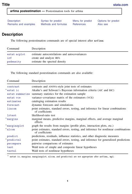
Description Syntax for predict Menu for predict Options for predict 

Remarks and examples Methods and formulas References Also see 

Description 

The following postestimation commands are of special interest after arfima: 

Command 

estat acplot 

irf 

psdensity 

Description 

estimate autocorrelations and autocovariances 

create and analyze IRFs 

estimate the spectral density 

The following standard postestimation commands are also available: 

Command Description 

contrast contrasts and ANOVA-style joint tests of estimates 

∗ estat ic Akaike’s and Schwarz’s Bayesian information criteria (AIC and BIC) 

estat summarize summary statistics for the estimation sample 

estat vce variance–covariance matrix of the estimators (VCE) 

estimates cataloging estimation results 

forecast dynamic forecasts and simulations 

lincom 

point estimates, standard errors, testing, and inference for linear combinations 

of coefficients 

lrtest 

likelihood-ratio test 

∗ margins marginal means, predictive margins, marginal effects, and average marginal 

effects 

∗ marginsplot graph the results from margins (profile plots, interaction plots, etc.) 

∗ nlcom 

point estimates, standard errors, testing, and inference for nonlinear combinations 

of coefficients 

predict predictions, residuals, influence statistics, and other diagnostic measures 

∗ predictnl point estimates, standard errors, testing, and inference for generalized predictions 

pwcompare pairwise comparisons of estimates 

test 

Wald tests of simple and composite linear hypotheses 

testnl 

Wald tests of nonlinear hypotheses 

∗ estat ic, margins, marginsplot, nlcom, and predictnl are not appropriate after arfima, mpl. 

1

2 arfima postestimation — Postestimation tools for arfima 

Syntax for predict 

predict [ type ] newvar [ if ] [ in ] [ , statistic options ] 

statistic 

Main 

xb 

residuals 

rstandard 

fdifference 

Description 

predicted values; the default 

predicted innovations 

standardized innovations 

fractionally differenced series 

These statistics are available both in and out of sample; type predict . . . if e(sample) . . . if wanted only for 

the estimation sample. 

options 

Options 

rmse( [ type ] newvar) 

dynamic(datetime) 

Description 

put the estimated root mean squared error of the predicted statistic 

in a new variable; only permitted with options xb and residuals 

forecast the time series starting at datetime; only permitted with 

option xb 

datetime is a # or a time literal, such as td(1jan1995) or tq(1995q1); see [D] datetime. 

Menu for predict 

Statistics > Postestimation > Predictions, residuals, etc. 

Options for predict 

✄ 

✄ Main 

xb, the default, calculates the predictions for the level of depvar. 

✄ 

residuals calculates the predicted innovations. 

rstandard calculates the standardized innovations. 

fdifference calculates the fractionally differenced predictions of depvar. 

✄ 

Options 

 

rmse( [ type ] newvar) puts the root mean squared errors of the predicted statistics into the specified 

new variables. The root mean squared errors measure the variances due to the disturbances but do 

not account for estimation error. rmse() is only permitted with the xb and residuals options. 

dynamic(datetime) specifies when predict starts producing dynamic forecasts. The specified datetime 

must be in the scale of the time variable specified in tsset, and the datetime must be 

inside a sample for which observations on the dependent variables are available. For example, dynamic(tq(2008q4)) 

causes dynamic predictions to begin in the fourth quarter of 2008, assuming 

that your time variable is quarterly; see [D] datetime. If the model contains exogenous variables, 

they must be present for the whole predicted sample. dynamic() may only be specified with xb.

arfima postestimation — Postestimation tools for arfima 3 

Remarks and examples 

Remarks are presented under the following headings: 

Forecasting after ARFIMA 

IRF results for ARFIMA 

stata.com 

Forecasting after ARFIMA 

We assume that you have already read [TS] arfima. In this section, we illustrate some of the 

features of predict after fitting an ARFIMA model using arfima. 

Example 1 

We have monthly data on the one-year Treasury bill secondary market rate imported from the 

Federal Reserve Bank (FRED) database using freduse; see Drukker (2006) and Stata YouTube video: 

Using freduse to download time-series data from the Federal Reserve for an introduction to freduse. 

Below we fit an ARFIMA model with two autoregressive terms and one moving-average term to the 

data.


. use http://www.stata-press.com/data/r13/tb1yr 

(FRED, 1-year treasury bill; secondary market rate, monthly 1959-2001) 

. arfima tb1yr, ar(1/2) ma(1) 

Iteration 0: log likelihood = -235.31856 

Iteration 1: log likelihood = -235.26104 (backed up) 









Refining estimates: 



ARFIMA regression 

Sample: 1959m7 - 2001m8 Number of obs = 506 

Wald chi2(4) = 1864.15 

Log likelihood = -235.11868 Prob > chi2 = 0.0000 

OIM 

tb1yr Coef. Std. Err. z P>|z| [95% Conf. Interval] 

tb1yr 

ARFIMA 

_cons 5.496709 2.920357 1.88 0.060 -.2270864 11.2205 

ar 

L1. .2326107 .1136655 2.05 0.041 .0098304 .4553911 

L2. .3885212 .0835665 4.65 0.000 .2247337 .5523086 

ma 

L1. .7755848 .0669562 11.58 0.000 .6443531 .9068166 

d .4606489 .0646542 7.12 0.000 .333929 .5873688 

/sigma2 .1466495 .009232 15.88 0.000 .1285551 .1647439 

Note: The test of the variance against zero is one sided, and the two-sided 

confidence interval is truncated at zero. 

All the parameters are statistically significant at the 5% level, and they indicate a high degree of 

dependence in the series. In fact, the confidence interval for the fractional-difference parameter d 

indicates that the series may be nonstationary. We will proceed as if the series is stationary and 

suppose that it is fractionally integrated of order 0.46. 

We begin our postestimation analysis by predicting the series in sample: 

. predict ptb 

(option xb assumed) 

We continue by using the estimated fractional-difference parameter to fractionally difference the 

original series and by plotting the original series, the predicted series, and the fractionally differenced 

series. See [TS] arfima for a definition of the fractional-difference operator.


. predict fdtb, fdifference 

. twoway tsline tb1yr ptb fdtb, legend(cols(1)) 

0 5 10 15 

1960m1 1970m1 1980m1 1990m1 2000m1 

month 

1−Year Treasury Bill: Secondary Market Rate 

xb prediction 

tb1yr fractionally differenced 

The above graph shows that the in-sample predictions appear to track the original series well and 

that the fractionally differenced series looks much more like a stationary series than does the original. 

Example 2 

In this example, we use the above estimates to produce a dynamic forecast and a confidence 

interval for the forecast for the one-year treasury bill rate and plot them. 

We begin by extending the dataset and using predict to put the dynamic forecast in the new 

ftb variable and the root mean squared error of the forecast in the new rtb variable. (As discussed 

in Methods and formulas, the root mean squared error of the forecast accounts for the idiosyncratic 

error but not for the estimation error.) 

. tsappend, add(12) 

. predict ftb, xb dynamic(tm(2001m9)) rmse(rtb) 

Now we compute a 90% confidence interval around the dynamic forecast and plot the original 

series, the in-sample forecast, the dynamic forecast, and the confidence interval of the dynamic 

forecast. 

. scalar z = invnormal(0.95) 

. generate lb = ftb - z*rtb if month>=tm(2001m9) 

(506 missing values generated) 

. generate ub = ftb + z*rtb if month>=tm(2001m9) 

(506 missing values generated) 

. twoway tsline tb1yr ftb if month>tm(1998m12) || 

> tsrline lb ub if month>=tm(2001m9), 

> legend(cols(1) label(3 "90% prediction interval"))


2 3 4 5 6 7 

1999m1 2000m1 2001m1 2002m1 

month 

1−Year Treasury Bill: Secondary Market Rate 

xb prediction, dynamic(tm(2001m9)) 

90% prediction interval 

IRF results for ARFIMA 

We assume that you have already read [TS] irf and [TS] irf create. In this section, we illustrate 

how to calculate the implulse–response function (IRF) of an ARFIMA model. 

Example 3 

Here we use the estimates obtained in example 1 to calculate the IRF of the ARFIMA model; see 

[TS] irf and [TS] irf create for more details about IRFs. 

. irf create arfima, step(50) set(myirf) 

(file myirf.irf created) 

(file myirf.irf now active) 

(file myirf.irf updated) 

. irf graph irf 

arfima, tb1yr, tb1yr 

1.5 

1 

.5 

0 

0 50 

step 

95% CI impulse−response function (irf) 

Graphs by irfname, impulse variable, and response variable


The figure shows that a shock to tb1yr causes an initial spike in tb1yr, after which the impact 

of the shock starts decaying slowly. This behavior is characteristic of long-memory processes. 

Methods and formulas 

Denote γ h , h = 1, . . . , t, to be the autocovariance function of the ARFIMA(p, d, q) process for 

two observations, y t and y t−h , h time periods apart. The covariance matrix V of the process of 

length T has a Toeplitz structure of 

⎛ 

γ 0 γ 1 γ 2 . . . γ 

⎞ 

T −1 

γ 1 γ 0 γ 1 . . . γ T −2 

V = ⎜ 

⎝ 

. 

. 

. 

. .. 

. ⎟ .. ⎠ 

γ T −1 γ T −2 γ T −3 . . . γ 0 

where the process variance is γ 0 = Var(y t ). We factor V = LDL ′ , where L is lower triangular and 

D = Diag(ν t ). The structure of L −1 is of importance. 

⎛ 

1 0 0 . . . 0 0 

⎞ 

−τ 1,1 1 0 . . . 0 0 

L −1 = 

−τ 2,2 −τ 2,1 1 . . . 0 0 

⎜ 

⎝ 

. 

. 

. 

. .. 

. .. 

. ⎟ .. ⎠ 

−τ T −1,T −1 −τ T −1,T −2 −τ T −1,T −2 . . . −τ T −1,1 1 

Let z t = y t − x t β. The best linear predictor of z t+1 based on z 1 , z 2 , . . . , z t is ẑ t+1 = 

∑ t 

k=1 τ t,kz t−k+1 . Define −τ t = (−τ t,t , −τ t,t−1 , . . . , −τ t−1,1 ) to be the tth row of L −1 up to, but 

not including, the diagonal. Then τ t = Vt 

−1 γ t , where V t is the t × t upper left submatrix of V and 

γ t = (γ 1 , γ 2 , . . . , γ t ) ′ . Hence, the best linear predictor of the innovations is computed as ̂ɛ = L −1 z, 

and the one-step predictions are ŷ = ̂ɛ + X̂β. In practice, the computation is 

ŷ = ̂L ( ) 

−1 y − X̂β + X̂β 

where ̂L and ̂V are computed from the maximum likelihood estimates. We use the Durbin–Levinson 

algorithm (Palma 2007; Golub and Van Loan 1996) to factor ̂V, invert ̂L, and scale y − X̂β using 

only the vector of estimated autocovariances ̂γ. 

The prediction error variances of the one-step predictions are computed recursively in the Durbin– 

Levinson algorithm. They are the ν t elements in the diagonal matrix D computed from the Cholesky 

factorization of V. The recursive formula is ν 0 = γ 0 , and ν t = ν t−1 (1 − τ 2 t,t). 

Forecasting is carried out as described by Beran (1994, sec. 8.7), ẑ T +k = ˜γ ′ ̂V k −1 ẑ, where 

˜γ ′ k = (̂γ T +k−1 , ̂γ T +k−2 , . . . , ̂γ k ). The forecast mean squared error is computed as MSE(ẑ T +k ) = ̂γ 0 − 

˜γ ′ ̂V −1˜γ k k . Computation of ̂V −1˜γ k is carried out efficiently using algorithm 4.7.2 of Golub and Van 

Loan (1996).


References 

Beran, J. 1994. Statistics for Long-Memory Processes. Boca Raton: Chapman & Hall/CRC. 

Drukker, D. M. 2006. Importing Federal Reserve economic data. Stata Journal 6: 384–386. 

Golub, G. H., and C. F. Van Loan. 1996. Matrix Computations. 3rd ed. Baltimore: Johns Hopkins University Press. 

Palma, W. 2007. Long-Memory Time Series: Theory and Methods. Hoboken, NJ: Wiley. 

Also see 

[TS] arfima — Autoregressive fractionally integrated moving-average models 

[TS] estat acplot — Plot parametric autocorrelation and autocovariance functions 

[TS] irf — Create and analyze IRFs, dynamic-multiplier functions, and FEVDs 

[TS] psdensity — Parametric spectral density estimation after arima, arfima, and ucm 

[U] 20 Estimation and postestimation commands

arfima postestimation - Stata

Create successful ePaper yourself

Delete template?

Save as template?