

xtnbreg postestimation - Stata
xtnbreg postestimation - Stata
xtnbreg postestimation - Stata

You also want an ePaper? Increase the reach of your titles
YUMPU automatically turns print PDFs into web optimized ePapers that Google loves.
Title<br />
stata.com<br />
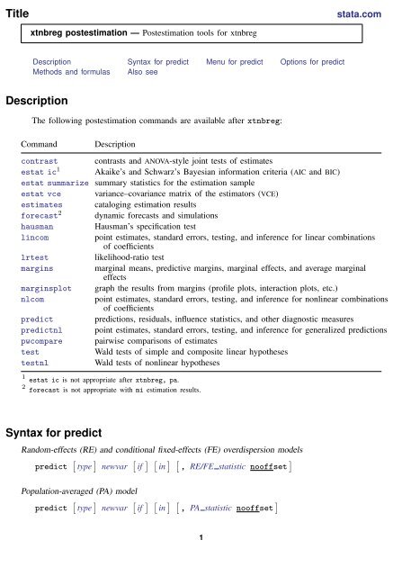
<strong>xtnbreg</strong> <strong>postestimation</strong> — Postestimation tools for <strong>xtnbreg</strong><br />
Description Syntax for predict Menu for predict Options for predict<br />
Methods and formulas Also see<br />
Description<br />
The following <strong>postestimation</strong> commands are available after <strong>xtnbreg</strong>:<br />
Command<br />
Description<br />
contrast contrasts and ANOVA-style joint tests of estimates<br />
estat ic 1 Akaike’s and Schwarz’s Bayesian information criteria (AIC and BIC)<br />
estat summarize summary statistics for the estimation sample<br />
estat vce variance–covariance matrix of the estimators (VCE)<br />
estimates cataloging estimation results<br />
forecast 2 dynamic forecasts and simulations<br />
hausman Hausman’s specification test<br />
lincom<br />
point estimates, standard errors, testing, and inference for linear combinations<br />
of coefficients<br />
lrtest<br />
likelihood-ratio test<br />
margins marginal means, predictive margins, marginal effects, and average marginal<br />
effects<br />
marginsplot graph the results from margins (profile plots, interaction plots, etc.)<br />
nlcom<br />
point estimates, standard errors, testing, and inference for nonlinear combinations<br />
of coefficients<br />
predict predictions, residuals, influence statistics, and other diagnostic measures<br />
predictnl point estimates, standard errors, testing, and inference for generalized predictions<br />
pwcompare pairwise comparisons of estimates<br />
test<br />
Wald tests of simple and composite linear hypotheses<br />
testnl<br />
Wald tests of nonlinear hypotheses<br />
1 estat ic is not appropriate after <strong>xtnbreg</strong>, pa.<br />
2 forecast is not appropriate with mi estimation results.<br />
Syntax for predict<br />
Random-effects (RE) and conditional fixed-effects (FE) overdispersion models<br />
predict [ type ] newvar [ if ] [ in ] [ , RE/FE statistic nooffset ]<br />
Population-averaged (PA) model<br />
predict [ type ] newvar [ if ] [ in ] [ , PA statistic nooffset ]<br />
1
2 <strong>xtnbreg</strong> <strong>postestimation</strong> — Postestimation tools for <strong>xtnbreg</strong><br />
RE/FE statistic<br />
Main<br />
xb<br />
stdp<br />
nu0<br />
iru0<br />
pr0(n)<br />
pr0(a,b)<br />
Description<br />
linear prediction; the default<br />
standard error of the linear prediction<br />
predicted number of events; assumes fixed or random effect is zero<br />
predicted incidence rate; assumes fixed or random effect is zero<br />
probability Pr(y j = n) assuming the random effect is zero;<br />
only allowed after <strong>xtnbreg</strong>, re<br />
probability Pr(a ≤ y j ≤ b) assuming the random effect is zero;<br />
only allowed after <strong>xtnbreg</strong>, re<br />
PA statistic<br />
Main<br />
mu<br />
rate<br />
xb<br />
stdp<br />
score<br />
Description<br />
predicted number of events; considers the offset(); the default<br />
predicted number of events<br />
linear prediction<br />
standard error of the linear prediction<br />
first derivative of the log likelihood with respect to x j β<br />
These statistics are available both in and out of sample; type predict . . . if e(sample) . . . if wanted only<br />
for the estimation sample.<br />
Menu for predict<br />
Statistics > Postestimation > Predictions, residuals, etc.<br />
Options for predict<br />
✄<br />
✄ <br />
Main<br />
<br />
xb calculates the linear prediction. This is the default for the random-effects and fixed-effects models.<br />
mu and rate both calculate the predicted number of events. mu takes into account the offset(), and<br />
rate ignores those adjustments. mu and rate are equivalent if you did not specify offset(). mu<br />
is the default for the population-averaged model.<br />
stdp calculates the standard error of the linear prediction.<br />
nu0 calculates the predicted number of events, assuming a zero random or fixed effect.<br />
iru0 calculates the predicted incidence rate, assuming a zero random or fixed effect.<br />
pr0(n) calculates the probability Pr(y j = n) assuming the random effect is zero, where n is a<br />
nonnegative integer that may be specified as a number or a variable (only allowed after <strong>xtnbreg</strong>,<br />
re).<br />
pr0(a,b) calculates the probability Pr(a ≤ y j ≤ b) assuming the random effect is zero, where a<br />
and b are nonnegative integers that may be specified as numbers or variables (only allowed after<br />
<strong>xtnbreg</strong>, re);
<strong>xtnbreg</strong> <strong>postestimation</strong> — Postestimation tools for <strong>xtnbreg</strong> 3<br />
b missing (b ≥ .) means +∞;<br />
pr0(20,.) calculates Pr(y j ≥ 20);<br />
pr0(20,b) calculates Pr(y j ≥ 20) in observations for which b ≥ . and calculates<br />
Pr(20 ≤ y j ≤ b) elsewhere.<br />
pr0(.,b) produces a syntax error. A missing value in an observation on the variable a causes a<br />
missing value in that observation for pr0(a,b).<br />
score calculates the equation-level score, u j = ∂ln L j (x j β)/∂(x j β).<br />
nooffset is relevant only if you specified offset(varname) for <strong>xtnbreg</strong>. It modifies the calculations<br />
made by predict so that they ignore the offset variable; the linear prediction is treated as x it β<br />
rather than x it β + offset it .<br />
Methods and formulas<br />
The probabilities calculated using the pr0(n) option are the probability Pr(y it = n) for a RE<br />
model assuming the random effect is zero. A negative binomial model is an overdispersed Poisson<br />
model, and the nominal overdispersion can be calculated as δ = s/(r − 1), where r and s are as<br />
given in the estimation results. Define µ it = exp(x it β + offset it ). Then the probabilities in pr0(n)<br />
are calculated as the probability that y it = n, where y it has a negative binomial distribution with<br />
mean δµ it and variance δ(1 + δ)µ it .<br />
Also see<br />
[XT] <strong>xtnbreg</strong> — Fixed-effects, random-effects, & population-averaged negative binomial models<br />
[U] 20 Estimation and <strong>postestimation</strong> commands


