

teffects nnmatch - Stata
teffects nnmatch - Stata
teffects nnmatch - Stata

You also want an ePaper? Increase the reach of your titles
YUMPU automatically turns print PDFs into web optimized ePapers that Google loves.
Title<br />
stata.com<br />
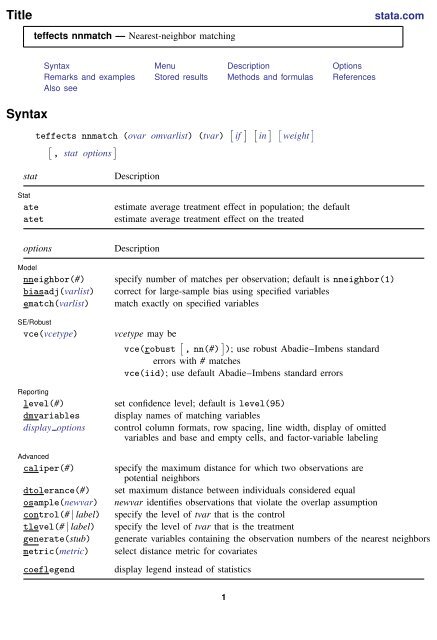
<strong>teffects</strong> <strong>nnmatch</strong> — Nearest-neighbor matching<br />
Syntax<br />
Syntax Menu Description Options<br />
Remarks and examples Stored results Methods and formulas References<br />
Also see<br />
<strong>teffects</strong> <strong>nnmatch</strong> (ovar omvarlist) (tvar) [ if ] [ in ] [ weight ]<br />
[<br />
, stat options<br />
]<br />
stat<br />
Stat<br />
ate<br />
atet<br />
Description<br />
estimate average treatment effect in population; the default<br />
estimate average treatment effect on the treated<br />
options<br />
Model<br />
nneighbor(#)<br />
biasadj(varlist)<br />
ematch(varlist)<br />
SE/Robust<br />
vce(vcetype)<br />
Reporting<br />
level(#)<br />
dmvariables<br />
display options<br />
Advanced<br />
caliper(#)<br />
dtolerance(#)<br />
osample(newvar)<br />
control(# | label)<br />
tlevel(# | label)<br />
generate(stub)<br />
metric(metric)<br />
coeflegend<br />
Description<br />
specify number of matches per observation; default is nneighbor(1)<br />
correct for large-sample bias using specified variables<br />
match exactly on specified variables<br />
vcetype may be<br />
vce(robust [ , nn(#) ] ); use robust Abadie–Imbens standard<br />
errors with # matches<br />
vce(iid); use default Abadie–Imbens standard errors<br />
set confidence level; default is level(95)<br />
display names of matching variables<br />
control column formats, row spacing, line width, display of omitted<br />
variables and base and empty cells, and factor-variable labeling<br />
specify the maximum distance for which two observations are<br />
potential neighbors<br />
set maximum distance between individuals considered equal<br />
newvar identifies observations that violate the overlap assumption<br />
specify the level of tvar that is the control<br />
specify the level of tvar that is the treatment<br />
generate variables containing the observation numbers of the nearest neighbors<br />
select distance metric for covariates<br />
display legend instead of statistics<br />
1
2 <strong>teffects</strong> <strong>nnmatch</strong> — Nearest-neighbor matching<br />
metric<br />
mahalanobis<br />
ivariance<br />
euclidean<br />
matrix matname<br />
Description<br />
inverse sample covariate covariance; the default<br />
inverse diagonal sample covariate covariance<br />
identity<br />
user-supplied scaling matrix<br />
Menu<br />
tvar must contain integer values representing the treatment levels.<br />
omvarlist may contain factor variables; see [U] 11.4.3 Factor variables.<br />
by and statsby are allowed; see [U] 11.1.10 Prefix commands.<br />
fweights are allowed; see [U] 11.1.6 weight.<br />
coeflegend does not appear in the dialog box.<br />
See [U] 20 Estimation and postestimation commands for more capabilities of estimation commands.<br />
Statistics > Treatment effects > Matching estimators > Nearest-neighbor matching<br />
Description<br />
<strong>teffects</strong> <strong>nnmatch</strong> estimates treatment effects from observational data by nearest-neighbor matching.<br />
NNM imputes the missing potential outcome for each subject by using an average of the outcomes<br />
of similar subjects that receive the other treatment level. Similarity between subjects is based on<br />
a weighted function of the covariates for each observation. The average treatment effect (ATE) is<br />
computed by taking the average of the difference between the observed and imputed potential outcomes<br />
for each subject.<br />
Options<br />
✄<br />
✄<br />
Model<br />
<br />
nneighbor(#) specifies the number of matches per observation. The default is nneighbor(1). Each<br />
observation is matched with at least the specified number of observations from the other treatment<br />
level. nneighbor() must specify an integer greater than or equal to 1 but no larger than the<br />
number of observations in the smallest treatment group.<br />
biasadj(varlist) specifies that a linear function of the specified covariates be used to correct for a<br />
large-sample bias that exists when matching on more than one continuous covariate. By default,<br />
no correction is performed.<br />
Abadie and Imbens (2006, 2011) show that nearest-neighbor matching estimators are not consistent<br />
when matching on two or more continuous covariates and propose a bias-corrected estimator that<br />
is consistent. The correction term uses a linear function of variables specified in biasadj(); see<br />
example 3.<br />
ematch(varlist) specifies that the variables in varlist match exactly. All variables in varlist must be<br />
numeric and may be specified as factors. <strong>teffects</strong> <strong>nnmatch</strong> exits with an error if any observations<br />
do not have the requested exact match.<br />
✄ <br />
✄ Stat<br />
stat is one of two statistics: ate or atet. ate is the default.<br />
ate specifies that the average treatment effect be estimated.<br />
atet specifies that the average treatment effect on the treated be estimated.
✄<br />
✄<br />
SE/Robust<br />
<br />
<strong>teffects</strong> <strong>nnmatch</strong> — Nearest-neighbor matching 3<br />
vce(vcetype) specifies the standard errors that are reported. By default, <strong>teffects</strong> <strong>nnmatch</strong> uses<br />
two matches in estimating the robust standard errors.<br />
vce(robust [ , nn(#) ] ) specifies that robust standard errors be reported and that the requested<br />
number of matches be used optionally.<br />
vce(iid) specifies that standard errors for independently and identically distributed data be<br />
reported.<br />
The standard derivative-based standard-error estimators cannot be used by <strong>teffects</strong> <strong>nnmatch</strong>,<br />
because these matching estimators are not differentiable. The implemented methods were derived<br />
by Abadie and Imbens (2006, 2011, 2012); see Methods and formulas.<br />
As discussed in Abadie and Imbens (2008), bootstrap estimators do not provide reliable standard<br />
errors for the estimator implemented by <strong>teffects</strong> <strong>nnmatch</strong>.<br />
✄ <br />
✄ Reporting<br />
level(#); see [R] estimation options.<br />
✄<br />
dmvariables specifies that the matching variables be displayed.<br />
display options: noomitted, vsquish, noemptycells, baselevels, allbaselevels, nofvlabel,<br />
fvwrap(#), fvwrapon(style), cformat(% fmt), pformat(% fmt), sformat(% fmt), and<br />
nolstretch; see [R] estimation options.<br />
✄<br />
Advanced<br />
<br />
caliper(#) specifies the maximum distance at which two observations are a potential match. By<br />
default, all observations are potential matches regardless of how dissimilar they are.<br />
The distance is based on omvarlist. If an observation has no matches, <strong>teffects</strong> <strong>nnmatch</strong> exits<br />
with an error.<br />
dtolerance(#) specifies the tolerance used to determine exact matches. The default value is<br />
dtolerance(sqrt(c(epsdouble))).<br />
Integer-valued variables are usually used for exact matching. The dtolerance() option is useful<br />
when continuous variables are used for exact matching.<br />
osample(newvar) specifies that indicator variable newvar be created to identify observations that<br />
violate the overlap assumption.<br />
control(# | label) specifies the level of tvar that is the control. The default is the first treatment<br />
level. You may specify the numeric level # (a nonnegative integer) or the label associated with<br />
the numeric level. control() and tlevel() may not specify the same treatment level.<br />
tlevel(# | label) specifies the level of tvar that is the treatment for the statistic atet. The default<br />
is the second treatment level. You may specify the numeric level # (a nonnegative integer) or<br />
the label associated with the numeric level. tlevel() may only be specified with statistic atet.<br />
tlevel() and control() may not specify the same treatment level.<br />
generate(stub) specifies that the observation numbers of the nearest neighbors be stored in the new<br />
variables stub1, stub2, . . . . This option is required if you wish to perform postestimation based<br />
on the matching results. The number of variables generated may be more than nneighbors(#)<br />
because of tied distances. These variables may not already exist.<br />
metric(metric) specifies the distance matrix used as the weight matrix in a quadratic form that<br />
transforms the multiple distances into a single distance measure; see Nearest-neighbor matching<br />
estimator in Methods and formulas for details.
4 <strong>teffects</strong> <strong>nnmatch</strong> — Nearest-neighbor matching<br />
The following option is available with <strong>teffects</strong> <strong>nnmatch</strong> but is not shown in the dialog box:<br />
coeflegend; see [R] estimation options.<br />
Remarks and examples<br />
stata.com<br />
The NNM method of treatment-effect estimation imputes the missing potential outcome for each<br />
individual by using an average of the outcomes of similar subjects that receive the other treatment level.<br />
Similarity between subjects is based on a weighted function of the covariates for each observation.<br />
The average treatment effect (ATE) is computed by taking the average of the difference between the<br />
observed and potential outcomes for each subject.<br />
<strong>teffects</strong> <strong>nnmatch</strong> determines the “nearest” by using a weighted function of the covariates for<br />
each observation. By default, the Mahalanobis distance is used, in which the weights are based on<br />
the inverse of the covariates’ variance–covariance matrix. <strong>teffects</strong> <strong>nnmatch</strong> also allows you to<br />
request exact matching for categorical covariates. For example, you may want to force all matches<br />
to be of the same gender or race.<br />
NNM is nonparametric in that no explicit functional form for either the outcome model or the<br />
treatment model is specified. This flexibility comes at a price; the estimator needs more data to get<br />
to the true value than an estimator that imposes a functional form. More formally, the NNM estimator<br />
converges to the true value at a rate slower than the parametric rate, which is the square root of<br />
the sample size, when matching on more than one continuous covariate. <strong>teffects</strong> <strong>nnmatch</strong> uses<br />
bias correction to fix this problem. <strong>teffects</strong> psmatch implements an alternative to bias correction;<br />
the method matches on a single continuous covariate, the estimated treatment probabilities. See<br />
[TE] <strong>teffects</strong> intro or [TE] <strong>teffects</strong> intro advanced for more information about this estimator.<br />
We will illustrate the use of <strong>teffects</strong> <strong>nnmatch</strong> by using data from a study of the effect of a<br />
mother’s smoking status during pregnancy (mbsmoke) on infant birthweight (bweight) as reported by<br />
Cattaneo (2010). This dataset also contains information about each mother’s age (mage), education<br />
level (medu), marital status (mmarried), whether the first prenatal exam occurred in the first trimester<br />
(prenatal1), whether this baby was the mother’s first birth (fbaby), and the father’s age (fage).<br />
Example 1: Estimating the ATE<br />
We begin by using <strong>teffects</strong> <strong>nnmatch</strong> to estimate the average treatment effect of mbsmoke<br />
on bweight. Subjects are matched using the Mahalanobis distance defined by covariates mage,<br />
prenatal1, mmarried, and fbaby.<br />
. use http://www.stata-press.com/data/r13/cattaneo2<br />
(Excerpt from Cattaneo (2010) Journal of Econometrics 155: 138-154)<br />
. <strong>teffects</strong> <strong>nnmatch</strong> (bweight mage prenatal1 mmarried fbaby) (mbsmoke)<br />
Treatment-effects estimation Number of obs = 4642<br />
Estimator : nearest-neighbor matching Matches: requested = 1<br />
Outcome model : matching min = 1<br />
Distance metric: Mahalanobis max = 139<br />
AI Robust<br />
bweight Coef. Std. Err. z P>|z| [95% Conf. Interval]<br />
ATE<br />
mbsmoke<br />
(smoker<br />
vs<br />
nonsmoker) -240.3306 28.43006 -8.45 0.000 -296.0525 -184.6087
<strong>teffects</strong> <strong>nnmatch</strong> — Nearest-neighbor matching 5<br />
Smoking causes infants’ birthweights to be reduced by an average of 240 grams.<br />
When the model includes indicator and categorical variables, you may want to restrict matches<br />
to only those subjects who are in the same category. The ematch() option of <strong>teffects</strong> <strong>nnmatch</strong><br />
allows you to specify such variables that must match exactly.<br />
Example 2: Exact matching<br />
Here we use the ematch() option to require exact matches on the binary variables prenatal1,<br />
mmarried, and fbaby. We also use Euclidean distance, rather than the default Mahalanobis distance,<br />
to match on the continuous variable mage, which uses Euclidean distance.<br />
. <strong>teffects</strong> <strong>nnmatch</strong> (bweight mage) (mbsmoke),<br />
> ematch(prenatal1 mmarried fbaby) metric(euclidean)<br />
Treatment-effects estimation Number of obs = 4642<br />
Estimator : nearest-neighbor matching Matches: requested = 1<br />
Outcome model : matching min = 1<br />
Distance metric: Euclidean max = 139<br />
AI Robust<br />
bweight Coef. Std. Err. z P>|z| [95% Conf. Interval]<br />
ATE<br />
mbsmoke<br />
(smoker<br />
vs<br />
nonsmoker) -240.3306 28.43006 -8.45 0.000 -296.0525 -184.6087<br />
Abadie and Imbens (2006, 2011) have shown that nearest-neighbor matching estimators are not<br />
consistent when matching on two or more continuous covariates. A bias-corrected estimator that uses<br />
a linear function of variables can be specified with biasadj().<br />
Example 3: Bias adjustment<br />
Here we match on two continuous variables, mage and fage, and we use the bias-adjusted estimator:<br />
. <strong>teffects</strong> <strong>nnmatch</strong> (bweight mage fage) (mbsmoke),<br />
> ematch(prenatal1 mmarried fbaby) biasadj(mage fage)<br />
Treatment-effects estimation Number of obs = 4642<br />
Estimator : nearest-neighbor matching Matches: requested = 1<br />
Outcome model : matching min = 1<br />
Distance metric: Mahalanobis max = 25<br />
AI Robust<br />
bweight Coef. Std. Err. z P>|z| [95% Conf. Interval]<br />
ATE<br />
mbsmoke<br />
(smoker<br />
vs<br />
nonsmoker) -223.8389 26.19973 -8.54 0.000 -275.1894 -172.4883
6 <strong>teffects</strong> <strong>nnmatch</strong> — Nearest-neighbor matching<br />
Stored results<br />
<strong>teffects</strong> <strong>nnmatch</strong> stores the following in e():<br />
Scalars<br />
e(N)<br />
e(nj)<br />
e(k levels)<br />
e(treated)<br />
e(control)<br />
e(k nneighbor)<br />
e(k nnmin)<br />
e(k nnmax)<br />
e(k robust)<br />
Macros<br />
e(cmd)<br />
e(cmdline)<br />
e(depvar)<br />
e(tvar)<br />
e(emvarlist)<br />
e(bavarlist)<br />
e(mvarlist)<br />
e(subcmd)<br />
e(metric)<br />
e(stat)<br />
e(wtype)<br />
e(wexp)<br />
e(title)<br />
e(tlevels)<br />
e(vce)<br />
e(vcetype)<br />
e(datasignature)<br />
e(datasignaturevars)<br />
e(properties)<br />
e(estat cmd)<br />
e(predict)<br />
e(marginsnotok)<br />
Matrices<br />
e(b)<br />
e(V)<br />
Functions<br />
e(sample)<br />
number of observations<br />
number of observations for treatment level j<br />
number of levels in treatment variable<br />
level of treatment variable defined as treated<br />
level of treatment variable defined as control<br />
requested number of matches<br />
minimum number of matches<br />
maximum number of matches<br />
matches for robust VCE<br />
<strong>teffects</strong><br />
command as typed<br />
name of outcome variable<br />
name of treatment variable<br />
exact match variables<br />
variables used in bias adjustment<br />
match variables<br />
<strong>nnmatch</strong><br />
mahalanobis, ivariance, euclidean, or matrix matname<br />
statistic estimated, ate or atet<br />
weight type<br />
weight expression<br />
title in estimation output<br />
levels of treatment variable<br />
vcetype specified in vce()<br />
title used to label Std. Err.<br />
the checksum<br />
variables used in calculation of checksum<br />
b V<br />
program used to implement estat<br />
program used to implement predict<br />
predictions disallowed by margins<br />
coefficient vector<br />
variance–covariance matrix of the estimators<br />
marks estimation sample<br />
Methods and formulas<br />
The methods and formulas presented here provide the technical details underlying the estimators<br />
implemented in <strong>teffects</strong> <strong>nnmatch</strong> and <strong>teffects</strong> psmatch. See Methods and formulas of [TE] <strong>teffects</strong><br />
aipw for the methods and formulas used by <strong>teffects</strong> aipw, <strong>teffects</strong> ipw, <strong>teffects</strong> ipwra,<br />
and <strong>teffects</strong> ra.<br />
Methods and formulas are presented under the following headings:<br />
Nearest-neighbor matching estimator<br />
Bias-corrected matching estimator<br />
Propensity-score matching estimator<br />
PSM, ATE, and ATET variance adjustment
<strong>teffects</strong> <strong>nnmatch</strong> — Nearest-neighbor matching 7<br />
Nearest-neighbor matching estimator<br />
<strong>teffects</strong> <strong>nnmatch</strong> implements the nearest-neighbor matching (NNM) estimator for the average<br />
treatment effect (ATE) and the average treatment effect on the treated (ATET). This estimator was<br />
derived by Abadie and Imbens (2006, 2011) and was previously implemented in <strong>Stata</strong> as discussed<br />
in Abadie et al. (2004).<br />
<strong>teffects</strong> psmatch implements nearest-neighbor matching on an estimated propensity score.<br />
A propensity score is a conditional probability of treatment. The standard errors implemented in<br />
<strong>teffects</strong> psmatch were derived by Abadie and Imbens (2012).<br />
<strong>teffects</strong> <strong>nnmatch</strong> and <strong>teffects</strong> psmatch permit two treatment levels: the treatment group<br />
with t = 1 and a control group with t = 0.<br />
Matching estimators are based on the potential-outcome model, in which each individual has<br />
a well-defined outcome for each treatment level; see [TE] <strong>teffects</strong> intro. In the binary-treatment<br />
potential-outcome model, y 1 is the potential outcome obtained by an individual if given treatmentlevel<br />
1 and y 0 is the potential outcome obtained by each individual i if given treatment-level 0. The<br />
problem posed by the potential-outcome model is that only y 1i or y 0i is observed, never both. y 0i<br />
and y 1i are realizations of the random variables y 0 and y 1 . Throughout this document, i subscripts<br />
denote realizations of the corresponding, unsubscripted random variables.<br />
Formally, the ATE is<br />
τ 1 = E(y 1 − y 0 )<br />
and the ATET is<br />
δ 1 = E(y 1 − y 0 |t = 1)<br />
These expressions imply that we must have some solution to the missing-data problem that arises<br />
because we only observe either y 1i or y 0i , not both.<br />
For each individual, NNM uses an average of the individuals that are most similar, but get the other<br />
treatment level, to predict the unobserved potential outcome. NNM uses the covariates {x 1 , x 2 , . . . , x p }<br />
to find the most similar individuals that get the other treatment level.<br />
More formally, consider the vector of covariates x i = {x i,1 , x i,2 , . . . , x i,p } and frequency weight<br />
w i for observation i. The distance between x i and x j is parameterized by the vector norm<br />
‖x i − x j ‖ S = {(x i − x j ) ′ S −1 (x i − x j )} 1/2<br />
where S is a given symmetric, positive-definite matrix.<br />
Using this distance definition, we find that the set of nearest-neighbor indices for observation i is<br />
Ω x m(i) = {j 1 , j 2 , . . . , j mi | t jk = 1 − t i , ‖x i − x jk ‖ S < ‖x i − x l ‖ S , t l = 1 − t i , l ≠ j k }<br />
Here m i is the smallest number such that the number of elements in each set, m i = |Ω x m(i)| =<br />
∑<br />
j∈Ω x m (i) w j, is at least m, the desired number of matches. You set the size of m using the<br />
nneighbors(#) option. The number of matches for the ith observation may not equal m because<br />
of ties or if there are not enough observations with a distance from observation i within the caliper<br />
limit, c, ‖x i − x j ‖ S ≤ c. You may set the caliper limit by using the caliper(#) option. For ease<br />
of notation, we will use the abbreviation Ω(i) = Ω x m(i).<br />
With the metric(string) option, you have three choices for the scaling matrix S: Mahalanobis,<br />
inverse variance, or Euclidean.
8 <strong>teffects</strong> <strong>nnmatch</strong> — Nearest-neighbor matching<br />
⎧<br />
⎪⎨<br />
S =<br />
diag<br />
⎪⎩<br />
(X − x ′ 1 n ) ′ W(X − x ′ 1 n )<br />
∑ n<br />
i w i − 1<br />
I p<br />
{ }<br />
(X − x ′ 1∑ n ) ′ W(X − x ′ 1 n )<br />
n w i i − 1<br />
if metric = mahalanobis<br />
if metric = ivariance<br />
if metric = euclidean<br />
where 1 n is an n × 1 vector of ones, I p is the identity matrix of order p, x = ( ∑ n<br />
i w ix i )/( ∑ n<br />
i w i),<br />
and W is an n × n diagonal matrix containing frequency weights.<br />
The NNM method predicting the potential outcome for the ith observation as a function of the<br />
observed y i is<br />
⎧<br />
y i if t i = t<br />
⎪⎨ ∑<br />
ŷ ti = wj y j<br />
j∈Ω(i)<br />
∑<br />
⎪⎩ wj<br />
otherwise<br />
for t ∈ {0, 1}.<br />
j∈Ω(i)<br />
We are now set to provide formulas for estimates ̂τ 1 , the ATE, and ̂δ 1 , the ATET,<br />
̂τ 1 =<br />
̂δ 1 =<br />
∑ n<br />
i=1 w i(ŷ 1i − ŷ 0i )<br />
∑ n<br />
i=1 w i<br />
=<br />
∑ n<br />
i=1 w i(2t i − 1){1 + K m (i)}y i<br />
∑ n<br />
i=1 w i<br />
∑ n<br />
i=1 t ∑ n<br />
iw i (ŷ 1i − ŷ 0i )<br />
∑<br />
i=1<br />
n<br />
i=1 t =<br />
{t i − (1 − t i )K m (i)}y<br />
∑ i<br />
n<br />
iw i i=1 t iw i<br />
where<br />
K m (i) = ∑<br />
j∈Ω(i)<br />
w j<br />
∑<br />
wk<br />
k∈Ω(j)<br />
The estimated variance of ̂τ 1 and ̂δ 1 are computed as<br />
̂σ 2 τ =<br />
̂σ 2 δ =<br />
∑ n<br />
[<br />
w i (ŷ 1i − ŷ 0i − ̂τ 1 ) 2 + ̂ξ<br />
]<br />
i 2 {Km(i) 2 + 2K m (i) − K m(i)}<br />
′<br />
i=1<br />
( ∑ n<br />
i=1 w i) 2<br />
∑ n<br />
[<br />
t iw i (ŷ 1i − ŷ 0i − ̂δ 1 ) 2 + ̂ξ<br />
]<br />
i 2 {Km(i) 2 − K m(i)}<br />
′<br />
i=1<br />
( ∑ n<br />
i=1 t iw i ) 2<br />
where<br />
K ′ m(i) = ∑<br />
j∈Ω(i)<br />
w j<br />
( ∑<br />
wk<br />
k∈Ω(j)<br />
) 2<br />
and ξ 2 i = var(y ti|x i ) is the conditional outcome variance. If we can assume that ξ 2 i does not vary<br />
with the covariates or treatment (homoskedastic), then we can compute an ATE estimate of ξ 2 τ as
<strong>teffects</strong> <strong>nnmatch</strong> — Nearest-neighbor matching 9<br />
̂ξ 2 τ =<br />
and an ATET estimate of ξ 2 δ as<br />
̂ξ 2 δ =<br />
1<br />
2 ∑ n<br />
i w i<br />
1<br />
2 ∑ n<br />
i t iw i<br />
⎡ ∑ ⎤<br />
wj {y n∑<br />
i − y j (1 − t i ) − ̂τ 1 } 2<br />
j∈Ω(i)<br />
w i<br />
⎢<br />
⎥<br />
⎣<br />
⎦<br />
i=1<br />
n ∑<br />
i=1<br />
∑<br />
wj<br />
j∈Ω(i)<br />
⎡ ∑<br />
tj w j {y i − y j (1 − t i ) − ̂δ<br />
⎤<br />
1 } 2<br />
j∈Ω(i)<br />
t i w i<br />
⎢<br />
⎣<br />
∑ ⎥<br />
tj w j<br />
⎦<br />
j∈Ω(i)<br />
If the conditional outcome variance is dependent on the covariates or treatment, we require an<br />
estimate for ξi<br />
2 at each observation. In this case, we require a second matching procedure, where we<br />
match on observations within the same treatment group.<br />
Define the within-treatment matching set<br />
Ψ x h(i) = {j 1 , j 2 , . . . , j hi | t jk = t i , ‖x i − x jk ‖ S < ‖x i − x l ‖ S , t l = t i , l ≠ j k }<br />
where h is the desired set size. As before, the number of elements in each set, h i = |Ψ x h<br />
(i)|, may<br />
vary depending on ties and the value of the caliper. You set h using the vce(robust, nn(#)) option.<br />
As before, we will use the abbreviation Ψ(i) = Ψ x h<br />
(i) where convenient.<br />
We estimate ξ 2 i<br />
by<br />
∑<br />
wj (y j − y Ψi ) 2<br />
̂ξ 2 t i<br />
(x i ) =<br />
j∈Ψ(i)<br />
∑<br />
wj − 1<br />
where y Ψi =<br />
j∈Ψ(i)<br />
∑<br />
wj y j<br />
j∈Ψ(i)<br />
∑<br />
wj − 1<br />
j∈Ψ(i)<br />
Bias-corrected matching estimator<br />
When matching on more than one continuous covariate, the matching estimator described above<br />
is biased, even in infinitely large samples; in other words, it is not √ n-consistent; see Abadie and<br />
Imbens (2006, 2011). Following Abadie and Imbens (2011) and Abadie et al. (2004), <strong>teffects</strong><br />
<strong>nnmatch</strong> makes an adjustment based on the regression functions µ t (˜x i ) = E(y t | ˜x = ˜x i ), for<br />
t = 0, 1 and the set of covariates ˜x i = (˜x i,1 , . . . , ˜x i,q ). The bias-correction covariates may be the<br />
same as the NNM covariates x i . We denote the least-squares estimates as ̂µ t (˜x i ) = ̂ν t + ̂β′ t˜x i, where<br />
we regress {y i | t i = t} onto {˜x i | t i = t} with weights w i K m (i), for t = 0, 1.<br />
Given the estimated regression functions, the bias-corrected predictions for the potential outcomes<br />
are computed as ⎧<br />
y i<br />
if t i = t<br />
⎪⎨ ∑<br />
ŷ ti = wj {y j + ̂µ t (˜x i ) − ̂µ t (˜x j )}<br />
j∈Ω<br />
⎪⎩<br />
x m (i) ∑<br />
wj − 1<br />
otherwise<br />
j∈Ω x m (i)<br />
The biasadj(varlist) option specifies the bias-adjustment covariates ˜x i .
10 <strong>teffects</strong> <strong>nnmatch</strong> — Nearest-neighbor matching<br />
Propensity-score matching estimator<br />
The propensity-score matching (PSM) estimator uses a treatment model (TM), p(z i , t, γ), to model<br />
the conditional probability that observation i receives treatment t given covariates z i . The literature<br />
calls p(z i , t, γ) a propensity score, and PSM matches on the estimated propensity scores.<br />
When matching on the estimated propensity score, the set of nearest-neighbor indices for observation<br />
i, i = 1, . . . , n, is<br />
Ω p m(i) = {j 1 , j 2 , . . . , j mi | t jk = 1 − t i , |̂p i (t) − ̂p jk (t)| < |̂p i (t) − ̂p l (t)|, t l = 1 − t i , l ≠ j k }<br />
where ̂p i (t) = p(z i , t, ̂γ). As was the case with the NNM estimator, m i is the smallest number such<br />
that the number of elements in each set, m i = |Ω p m(i)| = ∑ j∈Ω p m(i) w j, is at least m, the desired<br />
number of matches, set by the nneighbors(#) option.<br />
We define the within-treatment matching set analogously,<br />
Ψ p h (i) = {j 1, j 2 , . . . , j hi | t jk = t i , |̂p i (t) − ̂p jk (t)| < |̂p i (t) − ̂p l (t)|, t l = t i , l ≠ j k }<br />
where h is the desired number of within-treatment matches, and h i = |Ψ p h<br />
(i)|, for i = 1, . . . , n, may<br />
vary depending on ties and the value of the caliper. The sets Ψ p h<br />
(i) are required to compute standard<br />
errors for ̂τ 1 and ̂δ 1 .<br />
Once a matching set is computed for each observation, the potential-outcome mean, ATE, and ATET<br />
computations are identical to those of NNM. The ATE and ATET standard errors, however, must be<br />
adjusted because the TM parameters were estimated; see Abadie and Imbens (2012).<br />
PSM, ATE, and ATET variance adjustment<br />
The variances for ̂τ 1 and ̂δ 1 must be adjusted because we use ̂γ instead of γ. The adjusted variances<br />
for ̂τ 1 and ̂δ 1 have the following forms, respectively:<br />
̂σ 2 τ,adj = ̂σ 2 τ + ĉ ′ τ ̂V γ ĉ τ<br />
̂σ δ,adj 2 = ̂σ δ 2 − ĉ ′ ̂V δ γ ĉ δ + ̂∂δ 1 ̂V<br />
̂∂δ1<br />
∂γ ′ γ<br />
∂γ<br />
In both equations, the matrix ̂V γ is the TM coefficient variance–covariance matrix.<br />
The adjustment term for ATE can be expressed as<br />
ĉ τ =<br />
1<br />
∑ n<br />
i=1 w i<br />
n∑<br />
i=1<br />
( ĉov<br />
w i f(z ′ (zi , ŷ i1 )<br />
îγ)<br />
+ ĉov (z )<br />
i, ŷ i0 )<br />
̂p i (1) ̂p i (0)<br />
where<br />
f(z ′ îγ) = d p(z i, 1, ̂γ)<br />
d(z ′ îγ)
<strong>teffects</strong> <strong>nnmatch</strong> — Nearest-neighbor matching 11<br />
′<br />
is the derivative of p(z i , 1, ̂γ) with respect to z îγ, and<br />
⎧<br />
∑<br />
wj (z j − z Ψi )(y j − y Ψi )<br />
⎪⎨<br />
ĉov (z i , ŷ ti ) =<br />
⎪⎩<br />
is a p × 1 vector with<br />
j∈Ψ h (i)<br />
∑<br />
wj − 1<br />
j∈Ψ h (i)<br />
∑<br />
wj (z j − z Ωi )(y j − y Ωi )<br />
j∈Ω h (i)<br />
∑<br />
wj − 1<br />
j∈Ω h (i)<br />
if t i = t<br />
otherwise<br />
z Ψi =<br />
∑<br />
wj z j<br />
j∈Ψ h (i)<br />
∑<br />
wj<br />
z Ωi =<br />
∑<br />
wj z j<br />
j∈Ω h (i)<br />
∑<br />
wj<br />
and y Ωi =<br />
∑<br />
wj y j<br />
j∈Ω h (i)<br />
∑<br />
wj<br />
j∈Ψ h (i)<br />
j∈Ω h (i)<br />
j∈Ω h (i)<br />
Here we have used the notation Ψ h (i) = Ψ p h (i) and Ω h(i) = Ω p h<br />
(i) to stress that the within-treatment<br />
and opposite-treatment clusters used in computing ̂σ<br />
τ,adj 2 and ̂δ τ,adj 2 are based on h instead of the<br />
cluster Ω p m(i) based on m used to compute ̂τ 1 and ̂δ 1 , although you may desire to have h = m.<br />
The adjustment term c δ for the ATET estimate has two components, c δ = c δ,1 + c δ,2 , defined as<br />
c δ,1 =<br />
c δ,2 =<br />
1<br />
∑ n<br />
i=1 t iw i<br />
1<br />
∑ n<br />
i=1 t iw i<br />
n ∑<br />
i=1<br />
∑<br />
n<br />
i=1<br />
w i z i f(z ′ îγ)<br />
(ỹ 1i − ỹ 0i − ̂δ<br />
)<br />
1<br />
{<br />
w i f(z ′ îγ) ĉov (z i , ŷ 1i ) + ̂p }<br />
i(1)<br />
̂p i (0)ĉov (z i, ŷ 0i )<br />
where<br />
⎧ ∑<br />
wj y j<br />
j∈Ψ h (−i)<br />
∑<br />
wj<br />
⎪⎨ j∈Ψ h (−i)<br />
ỹ ti =<br />
∑<br />
wj y j<br />
if t = t i<br />
⎪⎩<br />
j∈Ω<br />
∑ h<br />
wj<br />
j∈Ω h<br />
otherwise<br />
and the within-treatment matching sets Ψ h (−i) = Ψ p h (−i) are similar to Ψp h<br />
(i) but exclude observation<br />
i:<br />
Ψ p h (−i) = {j 1, j 2 , . . . , j hi | j k ≠ i, t jk = t i , |̂p i − ̂p jk | < |̂p i − ̂p l |, t l = t i , l ∉ {i, j k }}<br />
Finally, we cover the computation of ∂γ ̂∂δ1 in the third term on the right-hand side of ̂σ 2 ′<br />
δ,adj . Here<br />
we require yet another clustering, but we match on the opposite treatment by using the covariates<br />
z i = (z i,1 , . . . , z i,p ) ′ . We will denote these cluster sets as Ω z m(i), for i = 1, . . . , n.<br />
The estimator of the p × 1 vector (∂δ 1 )/(∂γ ′ ) is computed as<br />
̂∂δ 1 1<br />
∂γ ′ = ∑ n<br />
i t iw i<br />
n ∑<br />
i=1<br />
z i f(z ′̂γ)<br />
{(2t i − 1)(y i − y Ω<br />
z<br />
m<br />
i) − ̂δ<br />
}<br />
1
12 <strong>teffects</strong> <strong>nnmatch</strong> — Nearest-neighbor matching<br />
where<br />
∑<br />
wj y j<br />
y Ω<br />
z<br />
m<br />
i<br />
=<br />
j∈Ω z m<br />
∑ (i)<br />
wj<br />
j∈Ω z m (i)<br />
References<br />
Abadie, A., D. M. Drukker, J. L. Herr, and G. W. Imbens. 2004. Implementing matching estimators for average<br />
treatment effects in <strong>Stata</strong>. <strong>Stata</strong> Journal 4: 290–311.<br />
Abadie, A., and G. W. Imbens. 2006. Large sample properties of matching estimators for average treatment effects.<br />
Econometrica 74: 235–267.<br />
. 2008. On the failure of the bootstrap for matching estimators. Econometrica 76: 1537–1557.<br />
. 2011. Bias-corrected matching estimators for average treatment effects. Journal of Business and Economic<br />
Statistics 29: 1–11.<br />
. 2012. Matching on the estimated propensity score. Harvard University and National Bureau of Economic<br />
Research. http://www.hks.harvard.edu/fs/aabadie/pscore.pdf.<br />
Cattaneo, M. D. 2010. Efficient semiparametric estimation of multi-valued treatment effects under ignorability. Journal<br />
of Econometrics 155: 138–154.<br />
Also see<br />
[TE] <strong>teffects</strong> postestimation — Postestimation tools for <strong>teffects</strong><br />
[TE] <strong>teffects</strong> — Treatment-effects estimation for observational data<br />
[TE] <strong>teffects</strong> psmatch — Propensity-score matching<br />
[U] 20 Estimation and postestimation commands


