teffects nnmatch - Stata
teffects nnmatch - Stata
teffects nnmatch - Stata
Create successful ePaper yourself
Turn your PDF publications into a flip-book with our unique Google optimized e-Paper software.
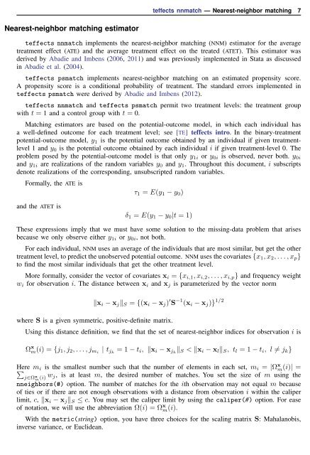
<strong>teffects</strong> <strong>nnmatch</strong> — Nearest-neighbor matching 7<br />
Nearest-neighbor matching estimator<br />
<strong>teffects</strong> <strong>nnmatch</strong> implements the nearest-neighbor matching (NNM) estimator for the average<br />
treatment effect (ATE) and the average treatment effect on the treated (ATET). This estimator was<br />
derived by Abadie and Imbens (2006, 2011) and was previously implemented in <strong>Stata</strong> as discussed<br />
in Abadie et al. (2004).<br />
<strong>teffects</strong> psmatch implements nearest-neighbor matching on an estimated propensity score.<br />
A propensity score is a conditional probability of treatment. The standard errors implemented in<br />
<strong>teffects</strong> psmatch were derived by Abadie and Imbens (2012).<br />
<strong>teffects</strong> <strong>nnmatch</strong> and <strong>teffects</strong> psmatch permit two treatment levels: the treatment group<br />
with t = 1 and a control group with t = 0.<br />
Matching estimators are based on the potential-outcome model, in which each individual has<br />
a well-defined outcome for each treatment level; see [TE] <strong>teffects</strong> intro. In the binary-treatment<br />
potential-outcome model, y 1 is the potential outcome obtained by an individual if given treatmentlevel<br />
1 and y 0 is the potential outcome obtained by each individual i if given treatment-level 0. The<br />
problem posed by the potential-outcome model is that only y 1i or y 0i is observed, never both. y 0i<br />
and y 1i are realizations of the random variables y 0 and y 1 . Throughout this document, i subscripts<br />
denote realizations of the corresponding, unsubscripted random variables.<br />
Formally, the ATE is<br />
τ 1 = E(y 1 − y 0 )<br />
and the ATET is<br />
δ 1 = E(y 1 − y 0 |t = 1)<br />
These expressions imply that we must have some solution to the missing-data problem that arises<br />
because we only observe either y 1i or y 0i , not both.<br />
For each individual, NNM uses an average of the individuals that are most similar, but get the other<br />
treatment level, to predict the unobserved potential outcome. NNM uses the covariates {x 1 , x 2 , . . . , x p }<br />
to find the most similar individuals that get the other treatment level.<br />
More formally, consider the vector of covariates x i = {x i,1 , x i,2 , . . . , x i,p } and frequency weight<br />
w i for observation i. The distance between x i and x j is parameterized by the vector norm<br />
‖x i − x j ‖ S = {(x i − x j ) ′ S −1 (x i − x j )} 1/2<br />
where S is a given symmetric, positive-definite matrix.<br />
Using this distance definition, we find that the set of nearest-neighbor indices for observation i is<br />
Ω x m(i) = {j 1 , j 2 , . . . , j mi | t jk = 1 − t i , ‖x i − x jk ‖ S < ‖x i − x l ‖ S , t l = 1 − t i , l ≠ j k }<br />
Here m i is the smallest number such that the number of elements in each set, m i = |Ω x m(i)| =<br />
∑<br />
j∈Ω x m (i) w j, is at least m, the desired number of matches. You set the size of m using the<br />
nneighbors(#) option. The number of matches for the ith observation may not equal m because<br />
of ties or if there are not enough observations with a distance from observation i within the caliper<br />
limit, c, ‖x i − x j ‖ S ≤ c. You may set the caliper limit by using the caliper(#) option. For ease<br />
of notation, we will use the abbreviation Ω(i) = Ω x m(i).<br />
With the metric(string) option, you have three choices for the scaling matrix S: Mahalanobis,<br />
inverse variance, or Euclidean.


