stcrreg postestimation - Stata

Title
stata.com
stcrreg postestimation — Postestimation tools for stcrreg
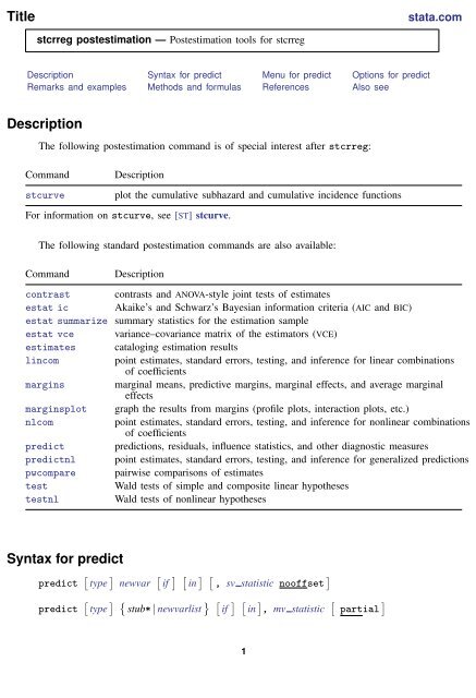
Description Syntax for predict Menu for predict Options for predict
Remarks and examples Methods and formulas References Also see
Description
The following postestimation command is of special interest after stcrreg:
Command Description
stcurve plot the cumulative subhazard and cumulative incidence functions
For information on stcurve, see [ST] stcurve.
The following standard postestimation commands are also available:
Command Description
contrast contrasts and ANOVA-style joint tests of estimates
estat ic Akaike’s and Schwarz’s Bayesian information criteria (AIC and BIC)
estat summarize summary statistics for the estimation sample
estat vce variance–covariance matrix of the estimators (VCE)
estimates cataloging estimation results
lincom
point estimates, standard errors, testing, and inference for linear combinations
of coefficients
margins marginal means, predictive margins, marginal effects, and average marginal
effects
marginsplot graph the results from margins (profile plots, interaction plots, etc.)
nlcom
point estimates, standard errors, testing, and inference for nonlinear combinations
of coefficients
predict predictions, residuals, influence statistics, and other diagnostic measures
predictnl point estimates, standard errors, testing, and inference for generalized predictions
pwcompare pairwise comparisons of estimates
test
Wald tests of simple and composite linear hypotheses
testnl
Wald tests of nonlinear hypotheses
Syntax for predict
predict [ type ] newvar [ if ] [ in ] [ , sv statistic nooffset ]
predict [ type ] { stub* | newvarlist } [ if ] [ in ] , mv statistic [ partial ]
1

2 stcrreg postestimation — Postestimation tools for stcrreg
sv statistic
Description
Main
shr
predicted subhazard ratio, also known as the relative subhazard; the default
xb
linear prediction x j β
stdp standard error of the linear prediction; SE(x j β)
∗ basecif baseline cumulative incidence function (CIF)
∗ basecshazard baseline cumulative subhazard function
∗ kmcensor Kaplan–Meier survivor curve for the censoring distribution
mv statistic
Main
∗ scores
∗ esr
∗ dfbeta
∗ schoenfeld
Description
pseudolikelihood scores
efficient score residuals
DFBETA measures of influence
Schoenfeld residuals
Unstarred statistics are available both in and out of sample; type predict . . . if e(sample) . . . if wanted only
for the estimation sample. Starred statistics are calculated only for the estimation sample, even when
if e(sample) is not specified.
nooffset is allowed only with unstarred statistics.
Menu for predict
Statistics > Postestimation > Predictions, residuals, etc.
Options for predict
✄
✄
Main
shr, the default, calculates the relative subhazard (subhazard ratio), that is, the exponentiated linear
prediction, exp(x j ̂β).
xb calculates the linear prediction from the fitted model. That is, you fit the model by estimating a
set of parameters, β 1 , β 2 , . . . , β k , and the linear prediction is ̂β 1 x 1j + ̂β 2 x 2j + · · · + ̂β k x kj , often
written in matrix notation as x j ̂β.
The x 1j , x 2j , . . . , x kj used in the calculation are obtained from the data currently in memory
and do not have to correspond to the data on the independent variables used in estimating β.
stdp calculates the standard error of the prediction, that is, the standard error of x j ̂β.
basecif calculates the baseline CIF. This is the CIF of the subdistribution for the cause-specific failure
process.
basecshazard calculates the baseline cumulative subhazard function. This is the cumulative hazard
function of the subdistribution for the cause-specific failure process.

stcrreg postestimation — Postestimation tools for stcrreg 3
kmcensor calculates the Kaplan–Meier survivor function for the censoring distribution. These estimates
are used to weight within risk pools observations that have experienced a competing event. As
such, these values are not predictions or diagnostics in the strict sense, but are provided for those
who wish to reproduce the pseudolikelihood calculations performed by stcrreg; see [ST] stcrreg.
nooffset is allowed only with shr, xb, and stdp, and is relevant only if you specified offset(varname)
for stcrreg. It modifies the calculations made by predict so that they ignore
the offset variable; the linear prediction is treated as x j ̂β rather than xj ̂β + offsetj .
scores calculates the pseudolikelihood scores for each regressor in the model. These scores are
components of the robust estimate of variance. For multiple-record data, by default only one score
per subject is calculated and it is placed on the last record for the subject.
Adding the partial option will produce partial scores, one for each record within subject;
see partial below. Partial pseudolikelihood scores are the additive contributions to a subject’s
overall pseudolikelihood score. In single-record data, the partial pseudolikelihood scores are the
pseudolikelihood scores.
One score variable is created for each regressor in the model; the first new variable corresponds
to the first regressor, the second to the second, and so on.
esr calculates the efficient score residuals for each regressor in the model. Efficient score residuals
are diagnostic measures equivalent to pseudolikelihood scores, with the exception that efficient
score residuals treat the censoring distribution (that used for weighting) as known rather than
estimated. For multiple-record data, by default only one score per subject is calculated and it is
placed on the last record for the subject.
Adding the partial option will produce partial efficient score residuals, one for each record
within subject; see partial below. Partial efficient score residuals are the additive contributions
to a subject’s overall efficient score residual. In single-record data, the partial efficient scores are
the efficient scores.
One efficient variable is created for each regressor in the model; the first new variable corresponds
to the first regressor, the second to the second, and so on.
dfbeta calculates the DFBETA measures of influence for each regressor of in the model. The DFBETA
value for a subject estimates the change in the regressor’s coefficient due to deletion of that subject.
For multiple-record data, by default only one value per subject is calculated and it is placed on
the last record for the subject.
Adding the partial option will produce partial DFBETAs, one for each record within subject; see
partial below. Partial DFBETAs are interpreted as effects due to deletion of individual records
rather than deletion of individual subjects. In single-record data, the partial DFBETAs are the
DFBETAs.
One DFBETA variable is created for each regressor in the model; the first new variable corresponds
to the first regressor, the second to the second, and so on.
schoenfeld calculates the Schoenfeld-like residuals. Schoenfeld-like residuals are diagnostic measures
analogous to Schoenfeld residuals in Cox regression. They compare a failed observation’s covariate
values to the (weighted) average covariate values for all those at risk at the time of failure.
Schoenfeld-like residuals are calculated only for those observations that end in failure; missing
values are produced otherwise.
One Schoenfeld residual variable is created for each regressor in the model; the first new variable
corresponds to the first regressor, the second to the second, and so on.

4 stcrreg postestimation — Postestimation tools for stcrreg
Note: The easiest way to use the preceding four options is, for example,
. predict double stub*, scores
where stub is a short name of your choosing. Stata then creates variables stub1, stub2, etc. You
may also specify each variable name explicitly, in which case there must be as many (and no
more) variables specified as there are regressors in the model.
partial is relevant only for multiple-record data and is valid with scores, esr, and dfbeta.
Specifying partial will produce “partial” versions of these statistics, where one value is calculated
for each record instead of one for each subject. The subjects are determined by the id() option
to stset.
Specify partial if you wish to perform diagnostics on individual records rather than on individual
subjects. For example, a partial DFBETA would be interpreted as the effect on a coefficient due to
deletion of one record, rather than the effect due to deletion of all records for a given subject.
Remarks and examples
stata.com
Remarks are presented under the following headings:
Baseline functions
Null models
Measures of influence
Baseline functions
Example 1: Cervical cancer study
In example 1 of [ST] stcrreg, we fit a proportional subhazards model on data from a cervical
cancer study.
. use http://www.stata-press.com/data/r13/hypoxia
(Hypoxia study)
. stset dftime, failure(failtype == 1)
(output omitted )
. stcrreg ifp tumsize pelnode, compete(failtype == 2)
(output omitted )
Competing-risks regression No. of obs = 109
No. of subjects = 109
Failure event : failtype == 1 No. failed = 33
Competing event: failtype == 2 No. competing = 17
No. censored = 59
Wald chi2(3) = 33.21
Log pseudolikelihood = -138.5308 Prob > chi2 = 0.0000
Robust
_t SHR Std. Err. z P>|z| [95% Conf. Interval]
ifp 1.033206 .0178938 1.89 0.059 .9987231 1.068879
tumsize 1.297332 .1271191 2.66 0.008 1.070646 1.572013
pelnode .4588124 .1972067 -1.81 0.070 .1975931 1.065365

stcrreg postestimation — Postestimation tools for stcrreg 5
After fitting the model, we can predict the baseline cumulative subhazard, H 1,0 (t), and the baseline
CIF, CIF 1,0 (t):
. predict bch, basecsh
. predict bcif, basecif
. list dftime failtype ifp tumsize pelnode bch bcif in 1/15
dftime failtype ifp tumsize pelnode bch bcif
1. 6.152 0 8 7 1 .0658792 .063756
2. 8.008 0 8.2 2 1 .0813224 .0781036
3. .003 1 8.6 10 1 .0260186 .025683
4. 1.073 1 3.3 8 1 .0379107 .0372011
5. .003 1 18.5 8 0 .0260186 .025683
6. 7.929 0 20 8 1 .0813224 .0781036
7. 8.454 0 21.8 4 1 .0813224 .0781036
8. 7.107 1 31.6 5 1 .0813224 .0781036
9. 8.378 0 16.5 5 1 .0813224 .0781036
10. 8.178 0 31.5 3 1 .0813224 .0781036
11. 3.395 0 18.5 4 1 .0658792 .063756
12. .003 1 12.8 5 0 .0260186 .025683
13. 1.35 1 18.4 4 1 .051079 .0497964
14. .003 1 18.5 8 1 .0260186 .025683
15. .512 2 21 10 0 .0260186 .025683
The baseline functions are for subjects who have zero-valued covariates, which in this example are
not representative of the data. If baseline is an extreme departure from the covariate patterns in your
data, then we recommend recentering your covariates to avoid numerical overflows when predicting
baseline functions; see Making baseline reasonable in [ST] stcox postestimation for more details.
For our data, baseline is close enough to not cause any numerical problems, but far enough to
not be of scientific interest (zero tumor size?). You can transform the baseline functions to those for
other covariate patterns according to the relationships
H 1 (t) = exp(xβ)H 1,0 (t)
and
CIF 1 (t) = 1 − exp{− exp(xβ)H 1,0 (t)}
but it is rare that you will ever have to do that. stcurve will predict, transform, and graph these
functions for you. When you use stcurve, you specify the covariate settings, and any you leave
unspecified are set at the mean over the data used in the estimation.

6 stcrreg postestimation — Postestimation tools for stcrreg
. stcurve, cif at1(ifp = 5 pelnode = 0) at2(ifp = 20 pelnode = 0)
Competing−risks regression
Cumulative Incidence
.1 .2 .3 .4 .5
0 2 4 6 8
analysis time
ifp = 5 pelnode = 0 ifp = 20 pelnode = 0
Because they were left unspecified, the cumulative incidence curves are for mean tumor size. If
you wish to graph cumulative subhazards instead of CIFs, use the stcurve option cumhaz in place
of cif.
Null models
Predicting baseline functions after fitting a null model (one without covariates) yields nonparametric
estimates of the cumulative subhazard and the CIF.
Example 2: HIV and SI as competing events
In example 4 of [ST] stcrreg, we analyzed the incidence of appearance of the SI HIV phenotype,
where a diagnosis of AIDS is a competing event. We modeled SI incidence in reference to a genetic
mutation indicated by the covariate ccr5. We compared two approaches: one that used stcrreg and
assumed that the subhazard of SI was proportional with respect to ccr5 versus one that used stcox
and assumed that the cause-specific hazards for both SI and AIDS were each proportional with respect
to ccr5. For both approaches, we produced cumulative incidence curves for SI comparing those who
did not have the mutation (ccr5==0) to those who did (ccr5==1).
To see which approach better fits these data, we now produce cumulative incidence curves that
make no model assumption about the effect of ccr5. We do this by fitting null models on the two
subsets of the data defined by ccr5 and predicting the baseline CIF for each. Because the models
have no covariates, the estimated baseline CIFs are nonparametric estimators.
. use http://www.stata-press.com/data/r13/hiv_si, clear
(HIV and SI as competing risks)
. stset time, failure(status == 2) // SI is the event of interest
(output omitted )

stcrreg postestimation — Postestimation tools for stcrreg 7
. stcrreg if !ccr5, compete(status == 1) noshow // AIDS is the competing event
Competing-risks regression No. of obs = 259
No. of subjects = 259
Failure event : status == 2 No. failed = 84
Competing event: status == 1 No. competing = 101
No. censored = 74
Wald chi2(0) = 0.00
Log pseudolikelihood = -435.80148 Prob > chi2 = .
Robust
_t SHR Std. Err. z P>|z| [95% Conf. Interval]
. predict cif_si_0, basecif
(65 missing values generated)
. label var cif_si_0 "ccr5 = 0"
. stcrreg if ccr5, compete(status == 1) noshow
Competing-risks regression No. of obs = 65
No. of subjects = 65
Failure event : status == 2 No. failed = 23
Competing event: status == 1 No. competing = 12
No. censored = 30
Wald chi2(0) = 0.00
Log pseudolikelihood = -88.306665 Prob > chi2 = .
Robust
_t SHR Std. Err. z P>|z| [95% Conf. Interval]
. predict cif_si_1, basecif
(259 missing values generated)
. label var cif_si_1 "ccr5 = 1"
. twoway line cif_si* _t if _t title(SI) ytitle(Cumulative Incidence) xtitle(analysis time)
SI
Cumulative Incidence
0 .1 .2 .3 .4
0 5 10 15
analysis time
ccr5 = 0 ccr5 = 1
After comparing with the graphs produced in [ST] stcrreg, we find that the nonparametric analysis
favors the stcox approach over the stcrreg approach.

8 stcrreg postestimation — Postestimation tools for stcrreg
Technical note
Predicting the baseline CIF after fitting a null model with stcrreg produces a nonparametric CIF
estimator that is asymptotically equivalent, but not exactly equal, to an alternate estimator that is
often used; see Coviello and Boggess (2004) for the details of that estimator. The estimator used by
predict after stcrreg is a competing-risks extension of the Nelson–Aalen estimator (Nelson 1972;
Aalen 1978); see Methods and formulas. The other is a competing-risks extension of the Kaplan–Meier
(1958) estimator.
In large samples with many failures, the difference is negligible.
Measures of influence
With predict after stcrreg, you can obtain pseudolikelihood scores that are used to calculate
robust estimates of variance, Schoenfeld residuals that reflect each failure’s contribution to the gradient
of the log pseudolikelihood, efficient score residuals that represent each subject’s (observation’s)
contribution to the gradient, and DFBETAs that measure the change in coefficients due to deletion of
a subject or observation.
Example 3: DFBETAs
Returning to our cervical cancer study, we obtain DFBETAs for each of the three coefficients in
the model and graph those for the first with respect to analysis time.
. use http://www.stata-press.com/data/r13/hypoxia, clear
(Hypoxia study)
. stset dftime, failure(failtype == 1)
(output omitted )
. stcrreg ifp tumsize pelnode, compete(failtype == 2)
(output omitted )
. predict df*, dfbeta
. generate obs = _n
. twoway scatter df1 dftime, yline(0) mlabel(obs)
DFBETA − ifp
−.006 −.004 −.002 0 .002 .004
31 37
94
1
21
47 86
57
100
70
186
15 22
24
29 30 88
79
106 107 102 80 45 3828
36 49 58
35 40 3253
50 26 2 9
54
51
56 11
60 61 76
63 62 72
96 109108 10397
75 89
25 33
59 16
55
64
66
68 81 83 98
91
93105
7
13
34 92 104 41 43
69 65
99
5 774267
78
39
90
10
23 52 27
17 10148
20
71
12
82
14
87
7419
85
73
3
95
44
4
46
0 2 4 6 8
Time from diagnosis to first failure or last follow−up (yrs)
84
8

stcrreg postestimation — Postestimation tools for stcrreg 9
predict created the variables df1, df2, and df3, holding DFBETA values for variables ifp,
tumsize, and pelnode, respectively. Based on the graph, we see that subject 4 is the most influential
on the coefficient for ifp, the first covariate in the model.
In the previous example, we had single-record data. If you have data with multiple records per
subject, then by default DFBETAs will be calculated at the subject level, with one value representing
each subject and measuring the effect of deleting all records for that subject. If you instead want
record-level DFBETAs that measure the change due to deleting single records within subjects, add the
partial option; see [ST] stcox postestimation for further details.
Methods and formulas
Continuing the discussion from Methods and formulas in [ST] stcrreg, the baseline cumulative
subhazard function is calculated as
Ĥ 1,0 (t) = ∑
j:t j≤t
The baseline CIF is ĈIF 1,0 (t) = 1 − exp{−Ĥ1,0(t)}.
δ j
∑
l∈R j
w l π lj exp(z l )
The Kaplan–Meier survivor curve for the censoring distribution is
Ŝ c (t) = ∏ { ∑
i
1 −
γ }
iI(t i = t (j) )
r(t (j) )
t (j)

10 stcrreg postestimation — Postestimation tools for stcrreg
Geskus, R. B. 2000. On the inclusion of prevalent cases in HIV/AIDS natural history studies through a marker-based
estimate of time since seroconversion. Statistics in Medicine 19: 1753–1769.
Kaplan, E. L., and P. Meier. 1958. Nonparametric estimation from incomplete observations. Journal of the American
Statistical Association 53: 457–481.
Milosevic, M., A. Fyles, D. Hedley, M. Pintilie, W. Levin, L. Manchul, and R. P. Hill. 2001. Interstitial fluid
pressure predicts survival in patients with cervix cancer independent of clinical prognostic factors and tumor oxygen
measurements. Cancer Research 61: 6400–6405.
Nelson, W. 1972. Theory and applications of hazard plotting for censored failure data. Technometrics 14: 945–966.
Pintilie, M. 2006. Competing Risks: A Practical Perspective. Chichester, UK: Wiley.
Putter, H., M. Fiocco, and R. B. Geskus. 2007. Tutorial in biostatistics: Competing risks and multi-state models.
Statistics in Medicine 26: 2389–2430.
Also see
[ST] stcrreg — Competing-risks regression
[ST] stcurve — Plot survivor, hazard, cumulative hazard, or cumulative incidence function
[U] 20 Estimation and postestimation commands